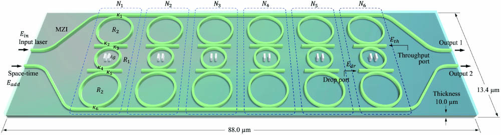
Fig. 1. Proposed design of the human-like micro stereo sensors system, where N₁ to N₆ are node 1 to node 6 for eye, ear, tongue, body, nose, and brain. R₁ and R₂ are radii of microring resonators. κ₁ to κ₄ are coupling coefficients. The optical fields for input, throughput, add, and drop ports are given by E_in, E_th, E_add, and E_dr, respectively.

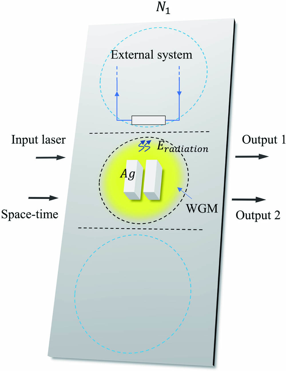
Fig. 2. Equivalent sensor node circuit. The center microring is embedded with a silver (Ag) nano bar.

Fig. 3. Illustration of OptiFDTD simulation results: (a) light intensity distribution and (b) electric field (plasmon) distribution. The input source is a polarized laser with a wavelength of 1.50 µm. The used parameters are given in Table 1.

Fig. 4. Plot of six sensor sensitivities with input power variation from 10 mW to 20 mW. The calculated sensor sensitivities obtained are 1.019 µm^-2, 0.722 µm^-2, 1.073 µm^-2, 0.239 µm^-2, 0.439 µm^-2, and 0.193 µm^-2, respectively.

Fig. 5. Plots of antenna parameters, where (a)–(f) are the directivities of antenna 1 to antenna 6. The obtained directivities are 2.91 dBm, 5.78 dBm, 4.92 dBm, 4.27 dBm, 3.51 dBm, and 8.14 dBm for antenna 1 to antenna 6, respectively, and (g) the gains of the antennas are 8.50 dB, 7.29 dB, 6.88 dB, 4.49 dB, 2.36 dB, and 3.30 dB of antenna 1 to antenna 6, respectively.

Fig. 6. WGM results of the sensor nodes in the frequency domain, where (a) to (f) are for node 1 to node 6, respectively.

Fig. 7. WGM results of the sensor nodes in the wavelength domain, where (a) to (f) are for node 1 to node 6, respectively.

Fig. 8. WGM results of the sensor nodes in the time domain, where (a) to (f) are for node 1 to node 6, respectively.

Fig. 9. Plots of the output signals of the six stereo sensor nodes (two-side ring results) with the optimum value from Fig. 4, where the upper small ring values are higher compared to the lower small ring.

Fig. 10. MZI output signals that describe the stereo sensors.

Fig. 11. Plots of electron density (ED) outputs with space–time control application: (a) ED and input power and (b) ED and time (phase).

Fig. 12. Two-level system results, where (a) one of the electron spin projection results, the quantum bit rate of 28 Pbit/s, is achieved, and (b) the Rabi oscillation gives the quantum behavior before collapsing at ∼1.4 fs.

Table 1. The Optimized Parameters Used in Simulation^{[19–26" target="_self" style="display: inline;">–26]}