Author Affiliations
1Key Laboratory of Intelligent Optical Sensing and Manipulation, Ministry of Education, Nanjing University, Nanjing 210023, Jiangsu , China2School of Optical and Electronic Information, Huazhong University of Science and Technology, Wuhan 430074, Hubei , China3Institute of Information Science, Beijing Jiaotong University, Beijing 100044, China4Research Center for Optical Fiber Sensing, Zhejiang Lab , Hangzhou 311100, Zhejiang , China5Key Laboratory of Optoelectronic Technology & Systems, Ministry of Education, Chongqing University,Chongqing 400044, China6School of Precision Instrument and Opto-Electronics Engineering, Tianjin University, Tianjin 300072, China7China Electric Power Research Institute, Beijing 100192, China8General Prospecting Institute of China National Administration of Coal Geology, Beijing 100039, China9Optical Science and Technology (Chengdu) Ltd., Chengdu 611731, Sichuan , China10Anhui Provincial Key Laboratory of Photonic Devices and Materials, Anhui Institute of Optics and Fine Mechanics, HFIPS, Chinese Academy of Science, Hefei 230031, Anhui , China11Qilu University of Technology (Shandong Academy of Sciences), Laser Institute, Shandong Academy of Sciences, Jinan 250104, Shandong , China12School of Aerospace Engineering, Xiamen University, Xiamen 361005, Fujian , China13School of Electric Information and Electrical Engineering, State Key Laboratory of Advanced Optical Communication Systems and Networks, Shanghai Jiao Tong University, Shanghai 200240, China14School of Optics and Photonics, MIIT Key Laboratory of Photonics Information Technology, Beijing Institute of Technology, Beijing 100081, China15Key Laboratory of Fiber Optic Sensing and Communication, Ministry of Education, University of Electronic Science and Technology of China, Chengdu 611731, Sichuan , China16College of Civil Engineering and Mechanics, Lanzhou University, Lanzhou 730000, Gansu , Chinashow less
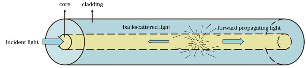
Fig. 1. Schematic diagram of transmission light scattering in optical fibers
Fig. 2. OTDR operating principle
Fig. 3. C-OTDR operating principle
Fig. 4. Φ-OTDR operating principle
Fig. 5. Principle diagrams of BOTDR and BOTDA. (a) BOTDR; (b) BOTDA
Fig. 6. Typical structure of ROTDR system (FUT: fiber under test; APD: avalanche photo diode; SpRS: spontaneous Raman scattering; WDM: wavelength division multiplexing)
Fig. 7. Schematic diagram of OFDR system
Fig. 8. Schematic diagram of DMI
Fig. 9. Schematic diagram of ADMZI
Fig. 10. Schematic diagrams of loop SI and in-line SI. (a) Schematic diagram of loop SI; (b) schematic diagram of in-line SI
Fig. 11. Schematic diagram of DOFS used in power system line monitoring
Fig. 12. Schematic diagram of distributed fiber optic sensing monitoring technology for coal mine geosafety
Fig. 13. Fiber optic monitoring, sound amplitude logging, and downhole TV results of borehole deformation damage process during grouting
Fig. 14. Schematic diagram of multi-field coupling and monitoring of geologic bodies
[203] Fig. 15. OptoSeisTM subsea permanent reservoir monitoring system layout and operation
Fig. 16. Surface 3D seismic data pre-stack depth migration (PSDM) imaging, underground three-component geophone array Walkaway VSP imaging, Walkaway DAS-VSP imaging, and corresponding amplitude spectra. (a) Surface 3D seismic data PSDM imaging and corresponding amplitude spectrum; (b) underground three-component geophone array Walkaway VSP imaging and corresponding amplitude spectrum; (c) Walkaway DAS-VSP imaging and corresponding amplitude spectrum
Fig. 17. Application diagram of distributed fiber optic sensing technology in transportation field
Fig. 18. Tunnel optical cable laying scheme and two-dimensional visualization data of temperature field
[209] Fig. 19. Train approaching construction personnel warning system schematic (top left image), and recognition results of the 63 km rail section from Mingguang to Chuzhou on the Beijing-Shanghai Line (top right and bottom images)
Fig. 20. Illustration of pipeline monitoring based on DOFS
Fig. 21. Applications of pipeline monitoring based on DOFS
[214-217] Fig. 22. Applications of DOFS in aerospace field
Fig. 23. Illustration of perimeter security monitoring based on DOFS system
Fig. 24. Applications of perimeter security monitoring. (a) Cable laying; (b) human intrusion; (c) monitoring interface and results
Fig. 25. Basic concept of hybrid DOFSs
Fig. 26. Typical setup for OTDR measurement on hollow-core fibers, OTDR measurement curves for anti-resonant hollow-core fibers,and sketch of flying particle distributed fiber sensor in hollow-core fibers. (a) Typical setup for OTDR measurement on hollow-core fibers
[308]; (b) OTDR measurement curves for anti-resonant hollow-core fibers
[309]; (c) sketch of flying particle distributed fiber sensor in hollow-core fibers
Fig. 27. Typical techniques and applications of machine learning in field of distributed optical fiber sensing
Fig. 28. Correlation analysis of optical fiber sensing signals and feature parameters of monitored structure
Fig. 29. Technical flow of intelligent characterization on physical state of monitored structure
Fig. 30. System configuration of double-digital comb based high spatial resolution
Φ-OTDR
[407] Fig. 31. Earthquake detection experimental setup using submarine optical fiber cable
[429] Fig. 32. Illustration of sensing system using submarine optical fiber cable
[432] Fig. 33. Principles of polarization-based seismic and water wave sensing
[433] Fig. 34. Integrated sensing and communication system in single optical fiber
[445] Fig. 35. Applications of fiber shape sensors. (a) Flexible wearable instrument based on optical fiber shape sensor; (b) soft robot based on optical fiber shape sensor; (c) fiber shape sensor in flexible instrument for intravascular navigation; (d) optical fiber sensor for wing shape sensing
Fig. 36. Schematic diagram of whale monitoring system based on DAS
[474] | Type | Technical principle | Performance | Ref. No |
|---|
| High spatial resolution | Pulse pre-pump | 5 cm@0.35 MHz@0.2 km 10 cm@0.35 MHz@1 km | [45-46] | | Differential pulse-width pair | 5 cm@50 m | [47] | | Long sensing distance | Distributed Raman/Brillouin amplifier | 8 m@2.06 MHz@175 km | [48-51] | | Optical pulse coding | 1 m@2.2 MHz@100.28 km | [52-55] | | High measurement accuracy | — | 2.5 m@0.55 MHz@62.3 km | [56-58] | | Dynamic measurement | Fast Fourier transform/short-time Fourier transform | 2 m@10 km | [59-60] | | Slope-assisted techniques | 2.5 m@2 km | [61-63] | | Frequency-agility modulation | 1 m@30 m | [64-65] | | Optical frequency comb | 12.5 m@10 km | [66-68] | | Multi-parameter measurement | Specialty optical fiber | 2 m@0.2 °C/9.7 µε@19.38 km | [69-72] |
|
Table 1. Summary of advanced BOTDR/BOTDA techniques
| Company | Sensing range / km | Spatial resolution /m | Temperature resolution /℃ | Time /s | Link |
|---|
| AP Sensing | 8 | ≥1 | 0.5 | — | https://www.apsensing.com/ | | SensorTran/Halliburton | 5-15 | 1-2 | 0.1-1.8 | 100 | https://www.halliburton.com/ | | IFOS | 5 | 1(3 km) | 1 | ≥120 | https://www.ifos.com/ | | LUNA/ LIOS | 10 | — | 1 | — | https://lios.lunainc.com/ | | Schlumberger | 4 | <1.2 | 0.1 | 30 | https://www.slb.com/ | | Sensornet/Nova Metrix | 15-45 | 1-5 | 2.25-2.75 | 10 | https://www.novavg.com/platforms/nova metrix/ | | Silixa | 10-35 | — | 0.01-0.1 | ≥1 | https://silixa.com/ | | Weatherford | 5-20 | 1.2 | 2.3(9760 m) | 40 | https://www.weatherford.com/ | | Yokogawa Electric | 6-50 | ≤1 | 0.02-2.6 | — | https://www.yokogawa.com/ | | Optromix | 16 | 0.5-4 | — | ≥10 | https://optromix.com/ | | Hangzhou Sensys Photonics | 4-16 | 0.5-3 | 0.2 | 1-10 | http://www.hzsensys.com/ | | Zhejiang ZhenDong | 2.5-16 | 0.5 | 0.2 | <2 | https://www.zdong.net/ | | Bandweaver | 2-40 | 1-5 | 0.1-1 | 240-600 | http://www.bandweaver.cn/index.php | | AGIOE | 2-30 | 1-5 | — | 1-30 | http://www.agioe.com/ | | Brillouin ε | 10 | 0.5-2 | 0.1 | 2.5 | http://www.buliyuan.com/ | | WUTOS | 10 | 1 | 2 | 1 | http://www.wutos.com/ |
|
Table 2. Summary of ROTDR manufacturers and their performance
| Methods | Performance |
|---|
| Nonlinear phase noise compensation methods | Hardware compensation[105] | Sensing distance:35 m;spatial resolution:22 μm | | | Resampling method[107] | Sensing distance:300 m;spatial resolution:0.3 mm | | | Concatenately generated phase method[112] | Sensing distance:40 km;spatial resolution:5 cm | | | Deskew filter method[109] | Sensing distance:80 km;spatial resolution:1.6 m | | | Increasing sensing distance methods | Highly linear swept fiber laser source[128] | Sensing distance:200 km | | Phase noise term detection[129] | Sensing distance:170 km | | Optical fiber delay loop compensation[130] | Sensing distance:30 km | | Improving strain/temperature range methods | Local spectral matching method[119] | Maximum strain:3000 με | | Machine learning prediction[117] | Maximum strain:2900 με | | Wavelet transform and Gaussian filtering[144] | Maximum strain:7000 µε | | Differential phase phase accumulation[132] | Maximum strain:3700 µε | | Femtosecond optical fiber grating[145] | Maximum temperature:1000 ℃ | | Annealed zirconia doped fiber[146] | Maximum temperature:800 ℃ | | Improving sensing resolution methods | Complex domain denoising[121] | Sensing resolution:0.89 mm | | Position offset compensation algorithm[103] | Sensing resolution:0.5 mm | | Total variational method and two-dimensional Gaussian filtering[136] | Sensing resolution:0.4 mm | | Improving dynamic measurement range methods | Time-frequency-multiplexing[141] | Maximum vibration frequency:33 kHz | | Phase demodulation algorithm[116] | Maximum vibration frequency:100 Hz | | Compressed sensing[145] | Maximum vibration frequency:40 Hz | | Time-gated digital OFDR[143] | Maximum vibration frequency:600 Hz |
|
Table 3. Summary of OFDR sensing performance improvement methods
| Parameter | Techniques | Applications |
|---|
| Acoustic signal | Φ-OTDR[214-217] | Threat detection and identification,micro-flow,flow | | Vibration | Sagnac interferometer[218],Mach-Zehnder interferometer[219] | Leak detection,pipeline pre-warning,intrusion detection | | Temperature | ROTDR[220],BOTDR[221],BOTDA[222] | Leakage location,micro-leakages,leak flow rate | | Strain | BOTDR[223],BOTDA[222],OFDR[223] | Buckling of pipeline,leakage of pipelines,pipeline corrosion and leakage |
|
Table 4. Overview of pipeline monitoring based on DOFS and its applications
| Applications | Specific scenarios | Measured & derived parameters | Types of DOFS and their indicators | Resources |
|---|
| Ground test and flight demonstration verification of civil aircraft | Flight verification of MU-300(climb,descend,and turn) | Measured:temperature and strain | BOCDA;indicators:spatial resolution of 30 mmanddynamic strain sampling rate of 27.8 Hz | Mitsubishi Heavy Industries,Ltd.(2014)[225] | | Composite head and wing box of airplane(landing,pressuring,and maneuvering) | Measured:temperature and strain; derived:disbond and impact | R-OFDR;indicators:spatial resolution of 5 mm/10 m | Airbus Defense and Space National Aerospace Laboratory of India[229] | | Manufacturing of composite structures | Measured:temperature and strain; derived:pressure | R-OFDR;indicators:spatial resolution of 2.6 mm,600 points,and sampling rate of 10 Hz | Imperial College London(2022) | | BOTDR and OTDR;optical fiber sensor embedded inside the composite laminate | The University of Tokyo(2012) | | Rocket component test | Cryogenic pressurization test of rocket fuel tanks | Measured:temperature and strain | OTDR;indicators:spatial resolution of 10 mm and strain sampling rate of 20 Hz | Xiamen University(2022)[234] | | Liquid rocket engines | Measured:temperature and strain; derived:heat flux and pressure | 3D printed integrated distributed sensors with OFDR;indicators:temperature range of -191-70 ℃,measurement accuracy of 3.6%-7.1%,and pressure range of 0-20.7 MPa | NASA and Luna(2020)[224] | | Smart sensing of spacecraft | Inflatable space habitats | Measured:strain | OTDR | NASA and Luna(2020)[230] | | Deformation reconstruction and shape sensing | Measured:strain; derived:displacement and distortion | OTDR | Italy and NASA,Dalian University of Technology (2021)[235] |
|
Table 5. Typical application scenarios and key indicators of distributed optical fiber sensing in aeronautic and aerospace fields
| Classification | Sub-system combination | Method for scattering light seperation | Method for performance enhancement | Fiber end access | Year |
|---|
| Combining Rayleigh and Brillouin scattering | POTDR/BOTDR[244] | Polarization switch | - | Single | 2013 | | Φ-OTDR/BOTDR[245] | Optical switch | Pulse modulation | Single | 2016 | | FS-Φ-OTDR/BOTDA[247] | FBG | Frequency-agile pulses | Double | 2020 | | | | | | | Φ-OTDR/BOTDA[249] | Space division multiplexing | - | Double | 2017 | | Φ-OTDR/BOTDA[250] | Wavelength division multiplexing | Distributed amplification technique | Double | 2018 | | Φ-OTDR/BOTDR[251] | Frequency division multiplexing | Double heterodyne detection | Single | 2022 | | TW-COTDR/BOTDA[253] | Not mentioned | Improved data processing | Double | 2014 | | COTDR/BOTDR[254] | Frequency division multiplexing | Coherent fading reduction | Single | 2021 | | FS-OTDR/BOTDA[268] | Wavelength division multiplexing | Enhanced slope-assisted method | Double | 2023 | | Φ-OTDR/single-end BOTDA[246] | Rayleigh backscattering as probe of BOTDA | Average | Single | 2023 | | Combining Rayleigh and Raman scattering | Φ-OTDR/ROTDR[256] | Raman filter | Cyclic Simplex coding | Single | 2016 | | Φ-OTDR/ROTDR[257] | Wavelength division multiplexing | Heterodyne detection | Single | 2018 | | Φ-OTDR/ROTDR[258] | Space division multiplexing | Wavelet transform denoising method | Single | 2018 | | Combining Brillouin and Raman scattering | BOTDR/ROTDR[269] | Wavelength division multiplexing | - | Single | 2004 | | BOTDA/ROTDR[260] | Raman filter | Cyclic Simplex coding | Double | 2013 | | BOTDR/ROTDR[261] | Space division multiplexing | - | Single | 2016 | | Combining Rayleigh Brillouin and Raman scattering | Φ-OTDR/single-end BOTDA/ROTDR[262] | Raman filter | Simplex coding | Single | 2023 |
|
Table 6. Recent advances of hybrid distributed optical fiber sensing systems
| Fiber type | G /dB | α /(dB/km) | Application system | Ref. No |
|---|
| Continous FBG | 14 | 0.4 | DAS | [270] | | Ge/B-doped fiber | 10 | >20000 | OFDR | [272] | | Er-doped fiber | - | - | DAS | [272] | | High-NA photonic crystal fiber | 12 | 3 | DTS/DAS | [273] |
|
Table 7. Enhancement factor G, fiber loss α, and application systems of different optical fiber types of continuous scattering enhancement
| Sensing cables | Technical characteristics | Ref. No |
|---|
| Highly thermal conductivity temperature sensing optical cables | Coated with a highly thermal conductivity composite material,i.e.,graphene for fast temperature sensing | [322] | | Highly thermal conductivity temperature sensing optical cable | Equipped with a highly thermal conductivity composite material jacket and tight cladding | [323] | | High temperature resistant measuring optical cable | Polyimide high temperature optical fiber is used,the middle is reinforced by Kevlar,and the outer sheath is protected by a layer of polytetrafluoroethylene | [324] | | Multi-core armored high-temperature resistant optical cable | Adopting a spiral armored tube and aramid braided structure,the working temperature range is -55-150 ℃. Preparation using high-temperature resistant engineering materials such as fluoroplastics | [325] | | High strength steel wire armored temperature sensing optical cable | Outer double steel wire twisted,sealed design,resistant to electrochemical corrosion,water and oil resistance,working temperature is -40-85 ℃ | [326] |
|
Table 8. Several typical structures of temperature sensing optical cables
| Sensing cables | Technical characteristics | Ref. No |
|---|
| Sensing fiber optic cable for distributed fiber optic strain measurement | Strengthen the protection of optical fibers through the design of equalizing fillers,and use equalizing fillers to evenly distribute the pressure at points | [327] | | Metal based cable | Metal based cable structure,optical fiber wrapped with metal reinforcement,thread structure based sensor surface | [194] | | Tightly sheathed sensing optical cable | Elastic modulus is small and should not be excessively stretched during the laying process | [194] | | Fiber reinforced multi-core strain sensing optical cable | Using glass fiber reinforced plastic(GFRP)reinforcement for protection,the overall elastic modulus is equivalent to that of concrete,and the strain transmission is good | [194] |
|
Table 9. Typical strain sensing optical cables
| Sensing cables | Technical characteristics | Ref. No |
|---|
| Variable winding pitch sensing optical cable | Fiber optic unit is wound around the center reinforcement to change the winding pitch and continuously spiral wound for placement | [328] | | Flexible sensing cables | Cables are designed and made with different reinforcement materials and structures. They have shown advantages such as small diameter,light weight,and flexibility while sensitivity being enhanced | [329] | | Vibration sensing cables | Inner wall of the outer sheath is fixedly connected with a wrapping tape,a reinforcing layer,a central bundle tube,and a colored optical fiber. The outer part of the colored optical fiber and the inner part of the central bundle tube are filled with ointment | [330] | | YOFC vibration sensing cables | Good flexibility,convenient construction of S-shaped laying,and good vibration sensitivity | [331] | | AP SENSING vibration sensing cables | Including metal tubes,non-metallic,sleeved or armored stainless steel | [332] |
|
Table 10. Typical vibration sensing optical cables
Signal type | Processing type | Institution | Multi-dimentional input | Model/method | Accuracy/ SNR enhancement | Application scenario | Publication date |
|---|
Single -source signal | Traditional machine learning | University of Electronic Science and Technology of China | Time | ANN | 94.4% | Pipeline | 2017[343] | | Shanghai Maritime University | T-F | PNN | 96.67% | Cable | 2018[344] | | Beijing Jiaotong University | Time | F-ELM | 95% | Perimeter | 2020[345] | | University of Alcala,Spain | Time | GMMs | 81.1% | Pipeline | 2016[346] | | University of Alcala,Spain | Time(long-short-term) | GMMs+HMM | 89.1% | Pipeline | 2019[347] | University of Electronic Science and Technology of China | Time(long-short-term) | HMM | 98.2% | Pipeline | 2019[348] | Deep learning | University of Electronic Science and Technology of China | Time | 1-D CNN | 98.19% | Pipeline | 2019[349] | Huazhong University of Science and Technology | Time | 1-D CNN + DenseNet | 98.4% | Cable | 2021[350] | | Beijing Jiaotong University | Time | DBN-GRU | 96.72% | Cable | 2023[351] | | UGES of Türkiye | T-F | 2-D CNN | 93% | Cable | 2017[352] | | Beijing Institute of Technology | T-F | 2-D CNN | 98.02% | Cable | 2018[353] | | Zhejiang University | T-F | 2-D CNN+SVM | 93.3% | Cable | 2018[354] | University of Electronic Science and Technology of China | T-F | Unsupervised SNN | 96.52% | Cable | 2021[355] | | Tongji University | T-S | 2-D CNN | 98% | Pipeline | 2020[356] | | Shantou University | T-S | Transfer learning | 96.16% | Cable | 2021[357] | | Tsinghua University | T-S | Semi-supervised learning(SSA) | 97.9% | Pipeline | 2021[358] | | Shanghai Institute of Optics and Fine Mechanics | S-F | DPN | 97% | Railway | 2019[359] | Multi-source aliasing signals | Enhancement/ separation | University of Electronic Science and Technology of China | — | Multi-scale wavelet decomposition | 28.42 dB | Perimeter security | 2015[360] | Anhui University and Nanjing University | — | Time delay estimation | — | Acoustic detection | 2017[361] | | Shanghai Institute of Optics and Fine Mechanics | — | Beamforming | 21 dB | Acoustic detection | 2020[362] | University of Electronic Science and Technology of China | — | FastICA | — | Cable | 2022[363] | | Tianjin University | — | Deep learning (TFA-DRNN) | — | Perimeter | 2022[364] |
|
Table 11. Intelligent signal processing methods and technical status at home and abroad of dynamic measurement DOFS
| Sensing solution | Improvement | Sensing range | Dynamic range | Spatial resolution | Ref. No |
|---|
| Multi-frequency probe pulse | Interference fading suppression | 10 km | - | 5 m | [400] | | Temporally sequenced multi-frequency probes | Extend the frequency measurement range | 9.6 km | 0.5 MHz | - | [405] | | Interrogating weak reflector array by using OFDM probes | Frequency response enhancement | 51 km | 25 kHz | 20.4 m | [406] | | Dual-comb spectrometry | Detection bandwidth reduction and spatial resolution improvement | 200 m | 20 Hz | 2 cm | [407] |
|
Table 12. Representative applications of frequency-division multiplexing techniques in Φ-OTDR system
| Sensing solution | Improvements | Sensing range | Spatial resolution | Frequency resolution | Measurement speed | Ref. No |
|---|
| Pump-probe pair | Scanning free | 2 km | 5 m | 3 MHz | 5.5 kHz | [401] | | Digital optical frequency comb | Dynamic range expansion | 10 km | 51.2 m | 1.95 MHz | 100 Hz | [67] | | Polarization-diversity frequency comb pump | Single-shot measurement | 10 km | 51.2 m | 1.95 MHz | 10 kHz | [408] | | Frequency comb and multiple pump pulses | Spatial resolution improvement | 10 km | 12.5 m | 2 MHz | 10 kHz | [409] | | Frequency comb and pump pulse array coding | Spatial resolution improvement | 9.5 km | 10.24 m | 2 MHz | 4.77 kHz | [410] | | Frequency-agility digital optical frequency comb | Spatial resolution improvement | 10 km | 5 m | 2 MHz | 40 Hz | [411] |
|
Table 13. Some important investigations of frequency-division multiplexed fast BOTDA
| Implementation scheme | Feature | Ref. No |
|---|
| Wavelength-division multiplexing | Flexible,with little cross-talk;but the sensing probe will occupy spectrum resources | [435-438] | | Frequency-division multiplexing | Flexible;but the sensing probe occupies spectrum resources and has cross-talk | [439-441] | | Mode-division multiplexing | Share the same wavelength,but might suffer from strong cross-talk | [442] | | Sensing using the received optical phase of communication signals | No additional sensing probe required,supporting long sensing range;but the positioning accuracy is bad | [434] | | Sensing using the backscattered light of communication signals | No additional sensing probe required;but special design on the communication signal and system is generally required | [443-445] |
|
Table 14. Configurations of communication and sensing hybrid systems
| Method | Sensor fiber | Sensing spatial resolution /mm | Error % |
|---|
| PPP-BOTDA[447] | SMF | 100 | 1.17 | | DPP-BOTDA[449] | MCF | 100 | 1 | | OFDR[454] | Fiber bundle | 1.907 | 0.58(2D) 3.45(3D) | | OFDR[455] | MCF+FBG array | 10 | 0.6(2D) 0.1(3D) | | OFDR[299] | Helical MCF | 1.5 | 0.4 | | Φ-OFDR[464] | MCF+PS array | 0.2 | 2.21(2D) 1.45(3D) |
|
Table 15. Summary of distributed optical fiber shape sensing methods