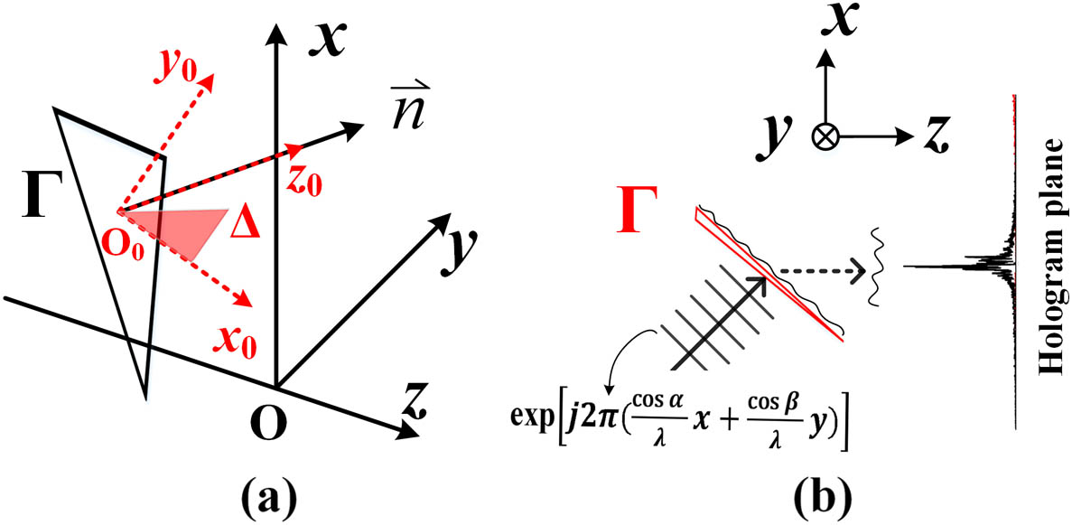
Fig. 1. Schematic of (a) affine transformation of two triangles and (b) triangular mesh diffraction with carrier wave.

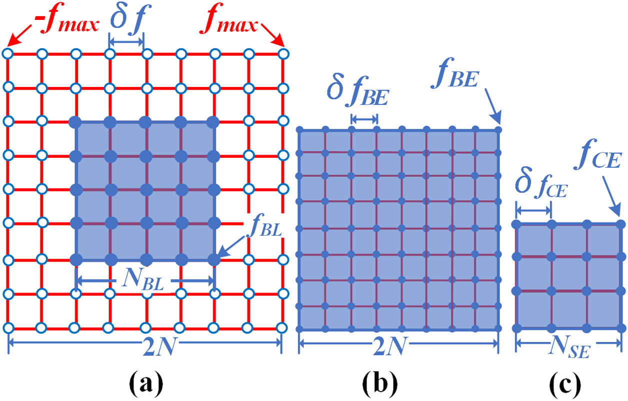
Fig. 2. Schematic diagram of the sampling strategy for (a) the band-limited, (b) the band-extended, and (c) the controllable energy angular spectrum methods. The blue areas are the effective bandwidth. The blue dots are the effective sampling points. The white circles are zero-padded. δf, δfBE, and δfCE are the sampling intervals of the three methods.

Fig. 3. (a) Rasterized triangle in the canvas under the parameters in Table 1. (b) Spectral energy density distributions at different frequency boundaries. (c) Normalized spectral energy distributions for different regions.

Fig. 4. Small triangle is defined as a reference triangle at the limiting angular resolution of the human eye.

Fig. 5. (a) Quality evaluation of the holograms obtained by the CE-ASM by PSNR (left) and SSIM (right) at different η values. The reference holograms are obtained by the BE-ASM with the expanded spectra. (b) Spectral range (left) and the number of sampling (right) of the CE-ASM on the x axis at different η values. The hologram has 1920×1080  pixels.

Fig. 6. (a) and (b) are holograms generated with the extended spectral region (BE-ASM) and the proposed compact spectral region (CE-ASM), respectively. (c) and (d) are the numerical reconstructions of (a) and (b), respectively. With the results of the extended spectral region as references, (b) and (d) show image quality by PSNR and SSIM.

Fig. 7. (a) Phong shading model: obtaining the normal of each pixel using linear interpolation based on three known vertex normals. (b) Schematic of interpolation of pixel normals within a triangle. (c) Blinn–Phong reflection model. L^ points along the direction of the light source. (d) Diffuse reflection diagram. (e) Specular reflection diagram.

Fig. 8. (a) Teapot with 1560 triangles and (b) rings with 5760 triangles located in the 3D space are illuminated by the light ray −L^ and observed with the vector −V^. (c) and (d) are reconstructed images of the teapot and rings rendered with the flat shading model, respectively.

Fig. 9. Schematic of continuous shading method without specular reflection proposed by Park et al. [32]. On the left is the spatial triangle in global coordinate system and on the right is the original triangle in local coordinate system. An affine transformation exists between them.

Fig. 10. Reconstructed results of Park et al.’s shading method (first column) and of the proposed sub-triangle-based shading method (columns 2 to 6). Teapot (a) and rings (b) are subdivided at M=2 to 6 in the proposed method. All results follow the Blinn–Phong reflection model and the parameters given in Table 3.

Fig. 11. Schematic of subdividing the mother triangle ΔABC at M=5, yielding 16 up sub-triangles and 9 down sub-triangles. ΔAB′C′ and ΔA′B′C′ are the original upper and lower sub-triangles, respectively.

Fig. 12. Efficiency comparison between the Park et al.’s method (solid line) and the proposed method (dashed line) at different values of M. From Fig. 11, M denotes the subdivision level of the mother triangle. The Park et al.’s method is independent of M; thus, it behaves as a constant as M increases.

Fig. 13. (a) Schematic diagram of backface culling and occlusion culling. (b) Schematic diagram of collision detection.

Fig. 14. Schematic diagram of an octree structure. A cube encloses the object, and then splits separately into eight children boxes. Empty boxes, such as boxes 2 and 3, and leaf boxes, such as box 7, stop splitting. However, the non-empty boxes (1 and 6) continue to split until a leaf box or empty box appears. Each leaf box contains a vertex set, which forms a set of triangles. The triangle set affiliated with a certain leaf box is the object of performing the intersection test.

Fig. 15. Reconstructed results by the proposed occlusion culling method. (a) Results of computing only the set of T0 triangles whose three vertices are visible. The teapot and ring were subdivided with M0=5 and M0=3, respectively, to smooth the shading. (b) Results of filling the set of T1 and T2 triangles after occlusion culling. (c) Reconstructed images from the optical experiments.

Fig. 16. Schematic diagram of occlusion culling. (a) Triangle set T1 with one vertex obscured and divided into M12 congruent sub-triangles. (b) Triangle set T2 with two vertices obscured and divided into M22 congruent sub-triangles. Blue sub-triangles are culled because they have at least one occluded vertex. (c)–(e) Three special cases that are occluded but cannot be properly addressed by the proposed method.

Fig. 17. Reconstructed images of all 3D objects referred in this paper. They are subjected to the proposed occlusion culling at the subdivision of M0,M1, and M2. The number of triangles for each object is given in Table 2. Shading rendering follows the method proposed in Section 4. (a) Numerically reconstructed images, and (b) experimentally reconstructed images.

Fig. 18. Flowchart of the proposed high-speed rendering pipeline for the polygon-based holograms.

Fig. 19. Numerical reconstruction of the ultra-high-resolution hologram of the Thai statue. The Thai statue contains 1,000,000 triangles and is subdivided by M0=M1=M2=3. The full running time in the pipeline is 607 s.

Table 1. Frequency Parameters of Different Sampling Methods

Table 2. Calculated Results and Comparison for Objects Composed of Different Numbers of Triangles

Table 3. Parameters Used in the Shading Model^a

Table 4. Elapsed Time Using the Proposed Occlusion Culling Method