As an important three-dimensional (3D) display technology, computer-generated holograms (CGHs) have been facing challenges of computational efficiency and realism. The polygon-based method, as the mainstream CGH algorithm, has been widely studied and improved over the past 20 years. However, few comprehensive and high-speed methods have been proposed. In this study, we propose an analytical spectrum method based on the principle of spectral energy concentration, which can achieve a speedup of nearly 30 times and generate high-resolution (8K) holograms with low memory requirements. Based on the Phong illumination model and the sub-triangles method, we propose a shading rendering algorithm to achieve a very smooth and realistic reconstruction with only a small increase in computational effort. Benefiting from the idea of triangular subdivision and octree structures, the proposed original occlusion culling scheme can closely crop the overlapping areas with almost no additional overhead, thus rendering a 3D parallax sense. With this, we built a comprehensive high-speed rendering pipeline of polygon-based holograms capable of computing any complex 3D object. Numerical and optical reconstructions confirmed the generalizability of the pipeline.
1. INTRODUCTION
Holography is a very promising technology in the field of real three-dimensional (3D) displays, as it is capable of reconstructing all depth information of 3D objects. Computer-generated holograms (CGHs) can simulate virtual objects, thereby providing opportunities for dynamic 3D displays and augmented reality interactions [1]. In CGHs, a single unit (point, polygon, or any other unit) affects all pixels in the hologram, which introduces huge computations. Therefore, efficient computing of holograms is essential for video-rate 3D displays. Many studies have reported efficient methods that fall into three main routes: point-based [2–4], layer-based [5–7], and polygon-based methods [8–14]. Notably, the line-based method reported in recent years employs a new computational idea that calculates only the contour lines of the object [15–17].
Point-based methods have rapidly developed owing to their computational simplicity. Lookup table methods [18], wavefront recording plane methods [19], parallel computation in graphics processing units (GPUs) [20], and field-programmable gate arrays [21] significantly improve the efficiency of point-based holograms. However, for a smooth and continuous complex 3D object, the computational effort versus the reconstructed image quality is still a trade-off [22]. Deep learning-generated holograms using layer-based RGBD data open exciting avenues for fewer calculations and higher quality [23–27]. Nevertheless, CGHs using deep learning do not simulate optical diffraction and interference processes, which may cause unwanted artifacts in scenes with a large range depth and hinder the generation of holograms in large fields of view [22]. The polygon-based method can render more realistic 3D scenes by drawing on computer graphics techniques, but it is computationally intensive because of the difficulty of simplifying calculations in the frequency domain [28].
The polygon-based method treats objects as a collection of triangular faces and has undergone a progression from spectral interpolation [8,9] to analytical spectral expression [10–14]. The former finds spectra by solving the fast Fourier transform (FFT) for the polygon and then interpolates the spectrum to obtain the spectrum distribution in the hologram plane. This easily renders the shading or texture information for individual polygons; however, each loop must perform one FFT and one interpolation, which is highly costly [28–30]. The spectral interpolation-based approach admittedly presents a highly realistic 3D viewing experience, especially by adding random phases to enable multi-viewing with full parallax [28,31], whereas this is more applicable to printed holograms using laser lithography rather than electronic display holograms. The analytic polygon-based method generally employs rotational transformation [10] or affine transformation [11–14] to derive an analytical spectral expression for an arbitrary triangle. The analytical expression significantly improves the computational performance of the polygon-based method because it does not require an FFT operation or interpolation. Nevertheless, individual triangles should be treated as having uniform transmittance, so detailed renderings such as shading require further subdivision surfaces, thus increasing the computational effort. Although researchers have reported some feasible solutions for presenting continuous shading without subdividing the objects [32,33], they either do not render specular reflection or add considerable additional overhead, as discussed in detail in Section 4.
Sign up for Photonics Research TOC. Get the latest issue of Photonics Research delivered right to you!Sign up now
In this study, we developed a comprehensive polygon-based hologram generation pipeline based on compact spectral regions and sub-triangulation, which essentially improves the computational efficiency of polygon-based holograms by rendering realistic reconstructed images. From the analysis of energy spectral density of the polygon [34], we observed that most spectral energy is concentrated in a small region with low frequency. Calculating only the low-frequency region can significantly accelerate the spectrum calculation, with little loss of quality in the hologram. For smooth objects, a shading model based on the surface normal is the fundamental path of shading. We propose a novel and simple shading method using the vertex-normal of sub-triangles, which can render very smooth shading without increasing the number of triangles.
In addition, the visibility culling technique is an important but challenging issue in CGH to obtain realistic 3D senses with motion parallax. Backface culling removes all backward triangles only [11,14], but not those facing forward, which may be occluded by groups of other objects in front of them. Occlusion culling is the most complex culling technique because it involves computing how objects (triangles) affect each other [35]. One candidate is the -buffer technique. However, this approach works in the point-based method [36,37], but not in the polygon-based method where each triangular surface is treated as a whole. For a polygon-based hologram, a few effective occlusion culling methods have been proposed: Matsushima et al. [38–40] proposed a silhouette method used for the interpolation-based algorithm, and Askari et al. [41] improved the silhouette method to enable its use in the analytical expression-based algorithm. Both methods require considerable additional computational effort.
To solve this problem, we propose a novel occlusion culling method for polygon-based holograms using the idea of sub-triangles. The proposed occlusion culling method adopts the concept of collision detection to determine whether the ray from the viewpoint to the detection point intersects with other triangles in the view frustum [35]. If it intersects, it is invisible; otherwise, it is visible. Because traversing all triangles for the intersection test is costly and redundant, we used an octree structure to quickly search for possible collision objects.
As an outline, in Section 2, the analytical spectral expression is briefly derived. In Section 3, the analytical spectrum is accelerated using the controllable energy angular spectrum method (CE-ASM) [42]. Based on the subdivision of triangles into up-and-down congruent triangles, we propose a fast shading method in Section 4 and an occlusion culling method in Section 5. In Section 6, we discuss the contributions and limitations of the proposed rendering pipeline. Finally, we present our conclusions in Section 7.
2. POLYGON-BASED HOLOGRAM
Full-analytical spectral methods for polygon-based holograms have been derived using several approaches [10–14]. In this study, we use the full-analytic method based on 3D affine transformation originating from Pan et al. [13,43]
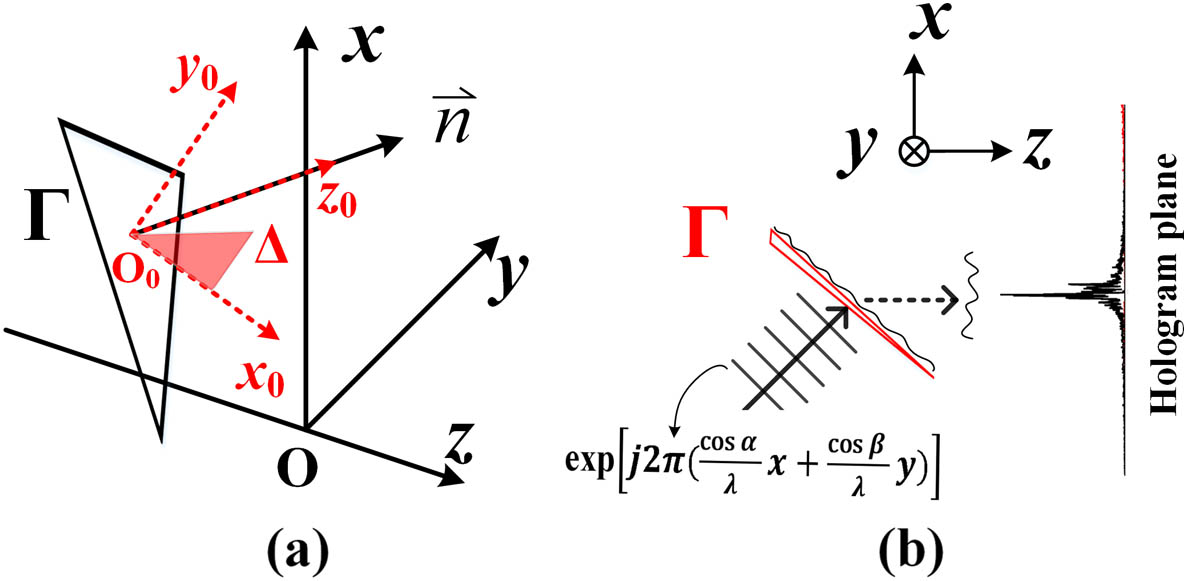
An arbitrary triangle in the global coordinate system is mapped onto a primitive triangle in the local coordinate system, as shown in Fig. 1(a). The affine transformation theory states that the mapping relationship between them is where represents the 3D affine transform and denotes the transpose. can be solved simply using ⏧where is a pseudo-inverse operation [42,44]. and are the vertex coordinate vectors of triangle and triangle , respectively. Let the vertices of triangle be and the vertices of primitive triangle be with (0, 0, 0), (0, 1, 0), and (1, 1, 0), where .
Figure 1.Schematic of (a) affine transformation of two triangles and (b) triangular mesh diffraction with carrier wave.
A plane light wave at angles and to the and axes, respectively, passes through the triangular polygon with a uniform transmittance, as shown in Fig. 1(b). The complex amplitude on the triangular surface is where is the wavelength, , and , where is the angle between the light source and axis. In general, we define a light source parallel to the axis, implying , and then .
In the frequency domain , the angular spectrum of is propagated to the hologram plane using the transfer function , where . Therefore, the spectra of the triangle in the hologram plane are where the vectors and . Based on the mapping relationship given in Eq. (1), the above equation can be further derived as where is the Jacobian factor, and the vectors and follow .
By integrating Eq. (5), we can obtain a fully analytic spectral expression as follows: where . Equation (6) is the diffractive spectrum of a single triangle on the hologram plane, indicating that it relates only to the affine transform matrix given in Eq. (2) and the frequency coordinates defined in the global system. It is noteworthy that Eq. (6) does not apply to cases such as or . Therefore, we suggest a tip to avoid conditional judgement in the program, plus a tiny value to the matrix , that is, , where .
Consequently, the hologram generated by an object with triangles is where denotes inverse Fourier transform. is the aggregate spectrum of all triangles, where is the spectrum of the th triangle obtained using Eq. (6). is the amplitude constant of the th triangle using which the shading in different illumination models can be controlled, as described in Section 4.
3. ACCELERATION: SPECTRAL ENERGY FOCUS METHOD
Although an accurate and fast hologram calculation from triangles is given in Section 2, this section proposes a method called the spectral energy focus method for faster calculation of accelerated holograms by skipping unwanted spectrum calculations.
A. Theorem
The diffraction based on the angular spectrum method (ASM) shown in Eq. (4) is a circular convolution process with a transfer function. To avoid edge errors caused by circular convolution, Matsushima and Shimobaba pointed out that the computational window should be calculated by double sampling [45]. However, at a position farther than the critical distance , where is the number of samples and is the sampling pitch, the high-frequency region cannot satisfy the Nyquist theorem because of the considerable oscillation of the transfer function of . The band-limited ASM (BL-ASM) proposed by Matsushima and Shimobaba [45] suggests a boundary frequency , such that the frequency of sampling in the region beyond is replaced by 0, as shown in Fig. 2(a). The blue area is the effective bandwidth within , and the external region of is zero-padded and is marked by white circles. The number of pixels in the calculation was whereas the effective number of samples was . The effective bandwidth shrinks rapidly with increasing diffraction distance, leading to a decrease in accuracy.
Figure 2.Schematic diagram of the sampling strategy for (a) the band-limited, (b) the band-extended, and (c) the controllable energy angular spectrum methods. The blue areas are the effective bandwidth. The blue dots are the effective sampling points. The white circles are zero-padded. , , and are the sampling intervals of the three methods.
Zhang et al. proposed a band-extended ASM (BE-ASM) with a boundary frequency [46]. As shown in Fig. 2(b), the BE-ASM provides a wider bandwidth and is more robust at a longer distance than the BL-ASM, which implies the highest accuracy of results. However, this requires substantial computational effort because of the full use of sampling.
Herein, the CE-ASM, we previously proposed, is used to accelerate the calculation of the polygon-based hologram [34], which involves a lighter load compared to BL-ASM and BE-ASM. The CE-ASM considers spectral energy in addition to the sampling theorem. For the triangular frequency spectrum , the energy spectral density is defined as . According to Parseval’s theorem [47], the energy of the frequency spectrum is where are the frequency boundaries. The full spectral energy of the triangle is , where is the maximum sampling frequency of the hologram. The spectral energies contained in BL-ASM and BE-ASM are and , respectively.
For a small triangle shown in Fig. 3(a), Fig. 3(b) presents its spectral energy density, a distribution with a central bulge and a flat surrounding. Different frequency boundaries enclose different regions, and the spectral energy within these regions can be calculated using Eq. (8) as shown in Fig. 3(c). The trend of Fig. 3(c) indicates that the spectral energy of the triangle is mainly focused on the low-frequency components, while the high-frequency component is negligible since the triangle is assumed to be uniform in amplitude. Therefore, we can obtain the vast majority of information by controlling a certain percentage of spectral energy.
Figure 3.(a) Rasterized triangle in the canvas under the parameters in Table 1. (b) Spectral energy density distributions at different frequency boundaries. (c) Normalized spectral energy distributions for different regions.
In the CE-ASM mentioned in Ref. [34], the frequency boundaries were determined based on the widest bandwidth because BE-ASM delivers an adequate reconstruction quality for considerably long propagation cases, such as tens of times the critical distance . In general, however, the CGH displayed in a spatial light modulator (SLM) is not propagated to that extent; in this work, considering the optical setup, a distance of 250 mm was used, which is approximately twice as long as under the parameters in Table 1. Therefore, in this study, we adopted as the basis for spectral energy; that is, the proposed new frequency boundaries satisfy where denotes a user-defined value. Above, implies that and always exist, which further indicates that the number of samples in the CE-ASM follows Then the sampling interval is A sampling schematic of the CE-ASM is shown in Fig. 2(c). The number of samples and the spectral region of the CE-ASM are smaller than those of the BL-ASM, which indicates that the computational effort of the proposed method can be reduced. The extent of the reduction depends on the value of , which will be discussed in detail in Section 3.B.
Frequency Parameters of Different Sampling Methods
Parameters
Values
Hologram pixels
Pixel pitch
μ
Physical size
Wavelength
Diffraction distance
Reference triangle
Vertices of the triangle
From the above, we can use to find the spectrum of the object using Eq. (6). However, the hologram cannot be obtained by executing an inverse FFT in Eq. (7) because is sampled at intervals of , which is inconsistent with the sampling pitch of the hologram . Therefore, a technique called non-uniform FFT (NUFFT) has been suggested for performing Eq. (7). NUFFT has been widely utilized to overcome the limitations of mismatched sampling intervals in the frequency and space domains [34,46,48]. Herein, we used the inverse type-3 NUFFT proposed by Lee and Greengard [49], where the hologram of the object is
B. Solving for the Frequency Sampling Boundary of CE-ASM
In Section 3.A, a compact spectral region, is deduced from Eq. (9), which is an approximate region that includes most of the spectral energy. However, an appropriate value of affects the energy within , which also implies that the quality of the hologram is lost because of the approximation.
First, we discuss reference spectral energy . Equation (8) indicates that the size of the reference triangle shown in Fig. 3(a), determines the effective spectral energy within . If the reference triangle is too small, a larger spectral region is involved; thus, the computational work is not significantly reduced. If it is large, the calculation can be accelerated, but the detailed representation of the 3D objects is lost. Therefore, for this trade-off, we analyzed the reference triangle in terms of visual acuity, which is a measurement of the eye’s ability to perceive details. The limit of the human eye for resolving two distinct points is 1′ of arc [50]. We assume an isosceles right triangle with a side length of as the reference triangle, which follows where denotes the distance from the viewer, as shown in Fig. 4. Therefore, the reference spectral energy can be obtained using this small reference right triangle.
Figure 4.Small triangle is defined as a reference triangle at the limiting angular resolution of the human eye.
Second, we analyzed the weight factor of the reference spectral energy in Eq. (9). is a custom value that depends on the quality of the hologram required by the user. Figure 5(a) shows the dependence of the hologram quality on the value, where the peak signal-to-noise ratio (PSNR) and structure similarity index (SSIM) are used to measure the hologram quality. Holograms were calculated using the parameters listed in Table 1. The reference hologram used as a metric was obtained by the BE-ASM under double sampling because the BE-ASM has the highest accuracy.
Figure 5.(a) Quality evaluation of the holograms obtained by the CE-ASM by PSNR (left) and SSIM (right) at different values. The reference holograms are obtained by the BE-ASM with the expanded spectra. (b) Spectral range (left) and the number of sampling (right) of the CE-ASM on the axis at different values. The hologram has .
From Fig. 5(a), the PSNR exceeds 35 dB and the SSIM stays above 0.9 when , which indicates that the value of is directly proportional to the quality. The boundary frequency and number of samples of the CE-ASM corresponding to different values of are shown in Fig. 5(b). From this, we can observe that the spectral region and number of samples increase with . When , and .
In general, images with a PSNR greater than 30 dB are considered acceptable because the human eye has a limited ability to recognize noise [51], and the highest quality of holographic displays in current experiments [24,27] is difficult to reach 30 dB. Therefore, to obtain higher quality holograms, we select as an energy threshold in all calculations below, with a PSNR of 37.5 dB and SSIM of 0.93. In this case, the hologram samples the spectral region of with the number of samples , reducing the number of samples by approximately 56 times at a high fidelity compared with the BE-ASM with the number of samples . Note that for higher-resolution holograms (such as 8K pixels), the BE-ASM requires a large amount of memory, which is difficult to achieve on a normal PC, whereas the proposed method requires very little memory owing to the compressed sampling.
The spectral region deduced by the CE-ASM is referred to as the compact spectra, whereas the spectral region deduced by the BE-ASM is referred to as the extended spectra.
C. Confirmed in Results
In this subsection, we confirm the principle and efficiency of the proposed compact spectral method by simulating concrete 3D objects.
Based on the parameters defined in Table 1 and the deduced , a hologram of a teapot model consisting of 1560 triangles located at with a depth of field of 5 mm was generated. Figures 6(a) and 6(b) show the holograms calculated using the extended spectra (BE-ASM) and compact spectra (CE-ASM), respectively, and Figs. 6(c) and 6(d) show the corresponding reconstructed images. The reconstructed image in Fig. 6(d) shows a negligible background apparition. Using the results of Figs. 6(a) and 6(c) as the references, PSNRs of the hologram and the reconstructed image are 44 dB and 40 dB, and their SSIMs are 0.95 and 0.92, respectively. This high fidelity demonstrated the effectiveness of the proposed method.
Figure 6.(a) and (b) are holograms generated with the extended spectral region (BE-ASM) and the proposed compact spectral region (CE-ASM), respectively. (c) and (d) are the numerical reconstructions of (a) and (b), respectively. With the results of the extended spectral region as references, (b) and (d) show image quality by PSNR and SSIM.
Notably, the actual number of triangles used for spectrum calculation is almost half of the total number because the backward triangles are easily recognized and removed by the surface normal. The very bright parts of the hologram in Fig. 6, such as the area indicated by dotted circles, are representations of the triangles overlapping each other, which requires occlusion culling, as discussed in Section 5. In addition, the amplitude of the reconstructed images was uniform because of the absence of illumination. The complex shading model is described in the following section.
In the computational environment of MATLAB 2021a, using a personal computer configured with CPU: AMD Ryzen 5-3600 at 3.59 GHz and GPU: Nvidia GeForce RTX 3070, we further calculated 3D objects with more triangles using the extended spectral region and the proposed compact spectral region. The computational efficiency values are listed in Table 2. Because the number of pixels used for the calculation in the compact spectral region is greatly reduced, the computational efficiency of the proposed method can be improved by a factor of approximately 30 as the number of polygons increases. Moreover, the PSNR and SSIM values of the holograms remained above 40 dB and 0.95, respectively. Thus, we conclude that the proposed compact spectral method is both efficient and accurate.
Calculated Results and Comparison for Objects Composed of Different Numbers of Triangles
Objects
Teapot
Rings
Hand
Soccer
Wang
Bunny
Angel
Number of triangles
1560
5760
8420
12,282
18,228
32,030
64,363
Extended spectra (s)
5.2
32.5
57.1
78.85
119.9
203.1
417.7
Compact spectra (s) (proposed)
0.4
1.2
2.0
2.70
4.0
6.6
13.7
Acceleration
14.1
26.0
28.6
29.2
29.8
30.8
30.5
PSNRa
44
45.1
42.4
46.2
51
46.3
47.4
SSIMa
0.95
0.97
0.96
0.97
0.99
0.96
0.97
The PSNR and SSIM listed here are only for holograms and not for the reconstructed images.
4. SMOOTH SHADING
A. Shading Model in Computer Graphics
Shading renders a photorealistic scene of 3D objects. The commonly used rendering model in computer graphics is the Phong shading model [52], which linearly interpolates the normal across the surface of the polygon. As shown in Fig. 7(a), based on known vertex normals (solid line arrows), the normal vectors of each pixel inside the surface (dashed arrows) are obtained by interpolation and then normalized. Figure 7(b) shows an interpolation schematic of a triangular surface based on the known normal vectors of the three vertices.
Figure 7.(a) Phong shading model: obtaining the normal of each pixel using linear interpolation based on three known vertex normals. (b) Schematic of interpolation of pixel normals within a triangle. (c) Blinn–Phong reflection model. points along the direction of the light source. (d) Diffuse reflection diagram. (e) Specular reflection diagram.
Under the illumination of incident light , as shown in Fig. 7(c), the amplitude of pixels on a polygon is obtained from a reflection model when viewed along the direction vector . In this study, we use the Blinn–Phong reflection model [53], which provides an equation for computing the amplitude of each surface point: where is the interpolated normal and denotes the unit vector. The vector denotes the reflected ray of at the point, which can be calculated using is defined as the halfway vector between the viewer and light-source vectors, calculated using which is a modification of the Phong reflection model. The constants , , and in Eq. (14) represent the ambient, diffuse, and specular reflection factors, respectively. Diffuse reflection depicts a rough surface that scatters the incident ray at many angles, as shown in Fig. 7(d). Specular reflection is the mirror-like reflection of light, which results in a significant effect on the surface along a specific angle, as shown in Fig. 7(e). The constant is the shininess factor of the material that determines the size of the specular highlight.
Figure 8.(a) Teapot with 1560 triangles and (b) rings with 5760 triangles located in the 3D space are illuminated by the light ray and observed with the vector . (c) and (d) are reconstructed images of the teapot and rings rendered with the flat shading model, respectively.
To address the Chevreul illusion, Park et al. developed an attractive continuous shading model that is essentially an extension of the Gouraud shading model, from interpolation of vertex amplitude to analytical spectra [32]. Park et al.’s shading method uses the reflection model which includes only the ambient and diffuse reflections, while the Blinn–Phong reflection model in Eq. (14) also includes the specular reflection. The triangle with known vertex normals , as shown in Fig. 9, is illuminated by the light . The reflection amplitude of the three vertices can be obtained using Eq. (17), defined as , , and . The amplitude of pixel within triangle satisfies the following interpolation expression: Because triangle is affine transformed into the right triangle in the local system described in Section 2 (see Fig. 1), the amplitude of pixel within the triangle defined in Eq. (7) is By substituting the above equation into Eqs. (4) and (5), the spectrum of triangle using integration operations is where is the same as in Eq. (6), and
Figure 9.Schematic of continuous shading method without specular reflection proposed by Park et al. [32]. On the left is the spatial triangle in global coordinate system and on the right is the original triangle in local coordinate system. An affine transformation exists between them.
Equation (20) provides a fully analytical expression with continuous shading at the cost of adding additional computational overhead to Eqs. (21) and (22). Although this cost is not significant, the weakness of Park et al.’s shading method is the absence of specular reflections, as shown in the first column of Fig. 10. As a comparison, Fig. 10 also shows the reconstructed results of the proposed sub-triangle-based shading method, which will be introduced below. From Fig. 10, Park et al.’s shading model lacks vividness due to the absence of highlights generated by specular reflection.
Figure 10.Reconstructed results of Park et al.’s shading method (first column) and of the proposed sub-triangle-based shading method (columns 2 to 6). Teapot (a) and rings (b) are subdivided at to 6 in the proposed method. All results follow the Blinn–Phong reflection model and the parameters given in Table 3.
B. Proposed Shading Model with Specular Reflection
Benefitting from the sub-triangle concept of Kim et al. [10], we propose an economical smooth shading method with specular reflection based on vertex normal interpolation of sub-triangles, unlike Park et al.’s shading method of interpolating pixel amplitude instead of normals [given in Eq. (18)]. Figure 11 shows a schematic of the subdivision of mother triangle . The vertices of the mother triangle are , and , and the known vertex normals are , and . Each side of the mother triangle is equally divided into segments, yielding sub-triangles, which include upper sub-triangles denoted and lower sub-triangles denoted . A non-orthogonal coordinate system is established with as -axis and as -axis. Each sub-triangle is then expressed as , which can be obtained by shifting the vertices of the original sub-triangle as follows: where denotes the three vertices of the sub-triangle, and and are the unit vectors of and axes, respectively. represents the vertex coordinates of the original sub-triangle, as shown in the upper-right corner of Fig. 11. Therefore, assuming that the spectrum of the original sub-triangle is which is calculated using Eq. (6), the spectrum of triangle is
Figure 11.Schematic of subdividing the mother triangle at , yielding 16 up sub-triangles and 9 down sub-triangles. and are the original upper and lower sub-triangles, respectively.
Similarly, the spectrum of triangle is is the spectrum of triangle . Because triangle is symmetric to triangle about side , there must exist a simple translation relationship. Therefore, can be calculated as where is the conjugate of .
Equations (24) and (25) indicate that the spectra of all sub-triangles can be directly obtained by simply shifting the spectrum of the original up sub-triangle . That is, regardless of the number of sub-triangles the mother triangle is subdivided into, we only need to calculate the spectrum of using Eq. (6). The concise computation was an improvement in Refs. [10,43].
Similar to the interpolation of the sub-triangle vertex coordinates in Eq. (18), vertex normals can also be obtained by interpolating the vertex normals of the mother triangle, , and . In this study, we used the average of the vertex normals as the face normal of the sub-triangles. Therefore, we define and as the face normals of triangles and , respectively, as follows: where and denote the normalized vectors. Based on the Blinn–Phong reflection model, the amplitudes of each sub-triangle, defined as and , are
Consequently, by combining Eqs. (24), (25), and (28), the spectrum of the th mother triangle in Eq. (7) with smooth shading, can be calculated as follows: which indicates that uniformly varying amplitudes are determined by the subdivision level of the mother triangle, i.e., the value of . Although the amplitude gradient is theoretically discontinuous, larger values result in a smoother rendering of the object surface. Figure 10 shows the reconstructed results of the teapot with 1560 triangles and rings with 5760 triangles for different values of . We can see that when , the reconstructed images of the teapot no longer exhibit a significant smoothness change, whereas for the rings, it does not change from . In Fig. 12, the dashed lines show the elapsed time of the proposed sub-triangle method at different values of . For comparison, the solid lines represent Park et al.’s method [32], which is independent of . From Fig. 12, as increases, the elapsed time of the proposed method will exceed that of Park et al.’s method. However, within the smoothing range perceptible to the human eye, we can choose an appropriate to allow the most economical calculation.
Figure 12.Efficiency comparison between the Park et al.’s method (solid line) and the proposed method (dashed line) at different values of . From Fig. 11, denotes the subdivision level of the mother triangle. The Park et al.’s method is independent of ; thus, it behaves as a constant as increases.
In summary, the sub-triangle shading method simulates the Phong shading model by replacing pixel normals with sub-triangle normals, which outperforms the method proposed by Park et al. [32] in terms of realistic rendering. Park et al.’s method uses the Gouraud shading model that interpolates pixel amplitude, and it also omits the specular reflection term, resulting in a loss of gloss. In terms of computational efficiency, the improved sub-triangle shading method simplifies the computational process, and thus also outperforms the traditional method of rendering by increasing the number of mother triangles [29,30] and the convolution-based method proposed by Yoem and Park [33].
5. OCCLUSION CULLING
A. Basic Mechanism of Occlusion Culling
Occlusion provides the most powerful monocular depth cues. As in all the reconstructed images shown in the previous sections, 3D objects appear as unusually bright areas because of the overlap of triangles along the same light of sight, such as the dashed circles in Fig. 6 and the interlocking rings shown in Fig. 10, which is known as incorrect occlusion.
In the polygon-based hologram, Matsushima et al. proposed an impressive method for occluded surface removal: the silhouette method [38–40]. However, the silhouette method requires the sorting of surfaces from front to back and at least two propagation processes for each surface, which is not economical. Askari et al. improved the silhouette method in the frequency domain using an analytical spectral expression [41], which avoids propagation twice and enhances the efficiency. However, this method employs three FFTs for each triangle. We argue that this is not very economical. In this section, we propose a novel occlusion culling method to effectively merge into the rendering pipeline of polygon-based holograms, while maintaining a full analytical frequency spectrum.
We first cull the backfaces that follow , where is the observation direction, , and is the surface normal. Assume that the 3D object has triangles, and forward triangles remain after performing backface culling. However, some forward triangles are still invisible, even if their normal points to the observer, such as multiple objects in front–back alignment, concave objects, and inter-occlusion triangles, as shown in Fig. 13(a). Therefore, we used collision detection to implement occlusion culling. Unlike computer graphics, where collisions are detected for each rasterized pixel, the proposed method performs collision detection for the vertices of all the forward triangles.
Figure 13.(a) Schematic diagram of backface culling and occlusion culling. (b) Schematic diagram of collision detection.
Figure 13(b) illustrates collision detection for . Detected vertices D, E, and F emit a ray into the hologram plane, and if this ray intersects a triangle, the vertex is occluded. Note that an orthogonal projection is used here, i.e., all the ray vectors are parallel to axis. Therefore, the task becomes a ray–triangle intersection test in geometry. In this study, we employ the intersection test algorithm optimized by Moller and Trumbore [56], hereafter referred to as where denotes the coordinate of the detected vertex, denotes the triangular set of potential occluders, denotes the unit vector of the ray, and . RayTriIntersect returns , implying that the vertex intersects one of the triangles, otherwise, “false”, implying no intersection. Generally, determining whether a vertex is occluded requires traversing all triangles and performing an intersection test. In other words, for triangles with vertices, the algorithm RayTriIntersect repeats times, which has significant redundancy.
B. Construct an Octree for Collision Detection
To avoid redundant queries for a more accurate intersection test, we developed an octree spatial data structure to organize the object geometry. An octree is a type of hierarchical structure, that is, the data are arranged at different levels from top to bottom. The topmost level contains eight children, each of which has its own eight or no children. For example, in Fig. 14, a cubical box that encloses the object is split into eight children boxes with the same size along the three axes, and each children box continues to split further into eight unless this box is empty or leaf. The leaf box is identified by certain criteria, such as reaching the maximum recursion depth or containing fewer than a certain number of vertices. The bottommost level of each stem is either a leaf box with some vertices or an empty box. The vertices in the leaf box are shared by some triangles; therefore, we consider that these triangles are affiliated with this leaf box.
Figure 14.Schematic diagram of an octree structure. A cube encloses the object, and then splits separately into eight children boxes. Empty boxes, such as boxes 2 and 3, and leaf boxes, such as box 7, stop splitting. However, the non-empty boxes (1 and 6) continue to split until a leaf box or empty box appears. Each leaf box contains a vertex set, which forms a set of triangles. The triangle set affiliated with a certain leaf box is the object of performing the intersection test.
In this study, we used a publicly available program to construct the octree data structure of 3D objects [57], hereafter referred to as where are the coordinates of all vertices, and property “leafCriteria” represents the criteria for being a leaf box. For example, a teapot consisting of 1560 triangles (containing 821 vertices) was divided into 441 boxes with up to five levels. The leaf box contained no more than 10 vertices. Suppose represents the th box located at the level, as shown in Fig. 14. If is an odd number, then the th box is the potential collision box of the th box. Conversely, if is an even number, there is no potential collision box at the level and the query should be directed to the level.
The hierarchical structure of the octree allows us to query potential collision boxes along the stem to the root rather than search through the entire object, which implies a reduction in performing the intersection test from times to times. During the query, as soon as a potential collision box appeared, the triangles affiliated with this box were immediately tested for intersections using Eq. (30). If the intersection with any triangle turns out to be “true,” the query is stopped, and the conclusion that this vertex is occluded is returned. In summary, the entire query is recursive in nature and ends in two cases: either the intersection test returns “true,” which means occlusion, or the query reaches the root, which means non-occlusion.
C. Occlusion Culling Based on Sub-Triangles
Collision detection returns the result of whether each vertex is occluded and the collision box if it is occluded. Among the triangles formed by these vertices, we classify them into four types: the first type is the fully visible triangle, i.e., none of the three vertices is occluded, defined as the set ; the second and third types are those with one and two invisible vertices, respectively, defined as the sets and , which are partially occluded; the fourth type is the fully invisible triangle, three vertices of which are occludees, defined as . Figure 15(a) shows the reconstruction results of only set for the teapot and rings, which appear fragmented because of the lack of partially occluded triangles. Therefore, the triangle sets and must be considered in the calculations.
Figure 15.Reconstructed results by the proposed occlusion culling method. (a) Results of computing only the set of triangles whose three vertices are visible. The teapot and ring were subdivided with and , respectively, to smooth the shading. (b) Results of filling the set of and triangles after occlusion culling. (c) Reconstructed images from the optical experiments.
In the case of occlusion culling for the triangle sets and , we follow the idea of subdividing the triangles presented in Section 4 to be able to use the analytic spectrum of triangles. Figure 16(a) shows two exemplary cases of triangles, and Fig. 16(b) shows two exemplary cases of triangles. Taking Fig. 16(a) as an example, is labeled as occludee after collision detection due to the invisibility of vertex A, and the corresponding collision box is . According to the description in Section 4, the occluded triangles are divided into congruent sub-triangles. For differentiation, we define as the subdivision of -type triangles, as the subdivision of -type triangles, and as the subdivision of -type triangles. The vertex coordinates of each sub-triangle can be solved using Eq. (23). Then, starting from vertex A, each sub-triangle vertex is again fed into the collision detection loop for the interaction test. If the vertex is obscured, all sub-triangles using this vertex are culled, as shown by the blue-shaded sub-triangles in Figs. 16(a)–16(d). Therefore, the final spectrum of the object should be the sum of the triangles retained after occlusion culling, expressed as where is the spectrum of the set of triangles, and and represent the spectrum after occlusion culling for the set of triangles and for the set of triangles, respectively. All terms in the above equation can be solved analytically using Eqs. (6) and (29).
Figure 16.Schematic diagram of occlusion culling. (a) Triangle set with one vertex obscured and divided into congruent sub-triangles. (b) Triangle set with two vertices obscured and divided into congruent sub-triangles. Blue sub-triangles are culled because they have at least one occluded vertex. (c)–(e) Three special cases that are occluded but cannot be properly addressed by the proposed method.
In summary, the proposed occlusion culling method removes some of the occluded sub-triangles from the sets of partially visible triangles and by continuing collision detection on the vertices of all sub-triangles. In this way, we cannot perfectly eliminate the occluded region along the boundary line, but we can adjust and to control the trajectory of the occlusion culling. Figure 15(b) shows the results of occlusion culling with for the teapot and for the rings. The edges of the occlusion appear very tight compared to those in Fig. 15(a), which confirms the proposed method. In addition, it should be noted that the proposed occlusion culling method does not apply to some exceptional cases: in Fig. 16(c), although the rear triangle is partially occluded, the collision detection mechanism cannot be triggered because all three vertices are visible; in Fig. 16(d), since all three vertices of the rear triangle are invisible, it is treated as fully invisible, although only the three angles are obscured; and in Fig. 16(e), two inlaid triangles occlude each other on the inside, but both are treated as fully visible. The proposed method can serve all the 3D models mentioned in this paper because they are closed, and there are no isolated groups of triangles. All 3D models were generated using the 3D modeling software Blender.
Figure 17(a) shows the numerically reconstructed images of all the 3D models mentioned in this paper after occlusion culling. The number of triangles and the shading rendering parameters of the objects are presented in Tables 2 and 3. The triangles , , and are subdivided by different values of , , and , respectively (see the legends). Each reconstructed image exhibited appropriate occlusion and a strong sense of realism in shading rendering, which confirms the generalizability of the proposed method. The supplementary Visualization 1 shows numerical reconstructions of three objects at different distances, where the objects automatically cull occlusions during rotation and apply constant illumination.
Figure 17.Reconstructed images of all 3D objects referred in this paper. They are subjected to the proposed occlusion culling at the subdivision of , and . The number of triangles for each object is given in Table 2. Shading rendering follows the method proposed in Section 4. (a) Numerically reconstructed images, and (b) experimentally reconstructed images.
Next, we discuss the efficiency of the proposed occlusion culling method. Table 4 lists the elapsed time for each object under occlusion culling. The three main added processes in the proposed method are octree construction, collision detection, and intersection tests of and sets. However, the proposed occlusion culling method incurs only a small extra cost compared to backface culling. This is because collision detection identifies triangles with all three vertices occluded while their surface normals face forward. These triangles do not require computation in occlusion culling, whereas they do so in backface culling. The increase in time consumed by the teapot is more pronounced because of the larger size of the occluded triangles, which requires more subdivision of the sub-triangles to sew them together tightly.
Elapsed Time Using the Proposed Occlusion Culling Method
Modelsa
Backface Culling Only (s)
Occlusion Culling (s)
Extra Costs
Octree
Detection
Total
Teapot
1.42
0.005
0.075
1.82
28.2%
Rings
3.79
0.02
0.13
4.23
11.6%
Hand
4.88
0.04
0.14
5.16
5.7%
Soccer
6.51
0.07
0.16
6.98
7.2%
Wang
9.94
0.10
0.42
10.86
9.3%
Bunny
21.78
0.54
1.18
23.53
8.0%
Angel
26.64
0.68
1.53
28.39
6.6%
The subdivision parameter is given in Fig. 17.
6. DISCUSSION
A. Contributions
Based on the fully analytic algorithm introduced in Section 2, we investigate three crucial aspects of generating polygon-based holograms from Sections 3–5: accelerated computation, shading rendering, and occlusion culling. These three aspects constitute a comprehensive, high-speed rendering pipeline for arbitrarily complex 3D objects. Figure 18 shows a full view of the rendering pipeline. First, the compact frequency sampling region , where the spectral energy is mainly concentrated, is calculated according to Section 3.A. The resampled frequency coordinates enter the pipeline and are used for subsequent analytical calculations. Second, backface culling of 3D objects was performed. If the remaining triangles are injected directly into the rendering pipeline, occlusion will result in a discordant brightness. Therefore, we performed collision detection using an octree structure to identify the occluded vertices. The set of fully visible triangles goes directly to the computation of the analytic spectrum. Then, shading rendering is activated with the Blinn–Phong reflection model according to the triangle subdivision method proposed in Section 4.B. For the partially occluded and sets, collision detection will continue for the subdivided triangle vertices until a fully visible sub-triangle is determined, and the shading is rendered in the same manner. Finally, all calculated triangle spectra are summed to obtain the diffraction spectrum of the object, and the hologram is obtained by performing the NUFFT given in Eq. (12).
Figure 18.Flowchart of the proposed high-speed rendering pipeline for the polygon-based holograms.
The holograms obtained by the proposed methods were encoded as a double phase [58] and imported into an SLM for optical reconstruction, as shown in Figs. 15(c) and 17(b), accordingly. The reconstructed images were displayed on a phase-only SLM with pixels (Jasper SRK4K) and captured by a camera (Sony ) at 250 mm from the SLM. The reconstructed images in the experiments show well a similar rendering to the simulated results, but some noise is always introduced due to the encoding. Several studies have suggested methods for the evaluation of hologram reconstructions and distortion correction [59,60]. To further demonstrate the generality of the proposed rendering pipeline, we imported a Thai statue model with one million triangles into the pipeline. A high-resolution hologram of 1 μm pixels was generated in approximately 10 minutes and reconstructed numerically, as shown in Fig. 19. All triangles are subdivided by , which means that the object contains a total of nine million sub-triangles. The reconstructed distance is at the front of the statue, whereas the rear appears blurry because it is out of focus. The animation of changing the focus position during reconstruction can be seen in Visualization 2. The supplementary Visualization 3 includes the reconstruction of the rotating Thai statue with occlusion culling. It is worth noting that online computing only takes up approximately 300 megabytes of memory for the GPU, but BE-ASM requires over 10 gigabytes of memory and takes approximately 5 h.
Figure 19.Numerical reconstruction of the ultra-high-resolution hologram of the Thai statue. The Thai statue contains 1,000,000 triangles and is subdivided by . The full running time in the pipeline is 607 s.
We have not been able to achieve real-time computation, but the primary problem is the use of MATLAB, and we believe that with full-scratch development using C++ and CUDA can be achieved in real time. Our proposed method is a lightweight algorithm owing to the analytical solution of the shading and occlusion processes using an octree. This computational complexity is less than that of the conventional method using FFTs and interpolation [9] and therefore has advantage in real-time computations.
The proposed rendering pipeline uses a certain degree of approximation at each session. Appropriate approximations perform very well in practical applications but seem to have limitations for more general situations. For example, although the spectral energy focus method skips unwanted spectrum calculations by controlling the value of given in Eq. (9), smaller values of lead to a lower reconstruction quality. In particular, shorter propagation spreads more spectral energy over the high-frequency components, which requires greater values of for fidelity and leads to a drop in acceleration. The values used to subdivide the mother triangles achieve different degrees of smooth shading, whereas excessive subdivision increases workload. Therefore, the appropriate can only be weighed empirically. Although the proposed occlusion culling method can eliminate the invisible localities of partially occlusions triangles, it is sometimes powerless, as shown in Figs. 16(c)–16(e).
The results of the in-focus and out-of-focus reconstruction of holograms confirmed monocular parallax, which is essential for 3D perception. However, objectively, the proposed CGH pipeline does not show reconstructions with motion parallax, that is, it fails to offer scenes viewed from multiple viewpoints. There are two reasons for the lack of motion parallax. First, the light wave emitted from the triangular mesh, as given in Eq. (3), propagates in a single direction so that illumination shading and occlusion culling will be processed only along this direction, and the other is the absence of a random phase assigned to each triangle leading to low-frequency signals that cannot spread to a larger field of view (FOV). By contrast, although the silhouette method [38–40] and its improved version [41] compromise computational lightness, they offer motion parallax for multiple viewpoints. Yeom et al.’s shading method [33] enables observation over a large FOV owing to the inclusion of multi-directional carrier waves through convolution calculations. For the proposed CGH pipeline, one way to address the problem of motion parallax or large FOV is to recalculate holograms from different viewpoints, including the particular carrier wave, shading reflection, and occlusion culling.
Alternatively, the light-field stereogram technique has a clear advantage in implementing full parallax [61–63], because it executes occlusion and shading processes for each viewpoint with well-refined 3D computer graphics techniques. Recently, light-field-based hologram calculations using deep learning have been proposed to achieve unparalleled image quality [27]. However, light field methods have the problem of requiring re-rendering for each element image, while the proposed polygon-based method is a timely rendering of the raw 3D object within the pipeline.
7. CONCLUSION
This study introduced a dedicated pipeline for computing polygon-based holograms and is capable of rendering realistic holograms with smooth shading at a high speed. The proposed pipeline involves three major novel methods, in which the compact sampling strategy for accelerating the computation is an extended application of that proposed in the authors’ previous publications [34]. The triangle subdivision method improves smooth rendering, particularly the specular effect that has not yet been considered in other studies [10,43], and the sub-triangle-based occlusion culling method is pioneering.
Compact spectra were adopted to narrow the sampling range using energy-focused approximation. Although we discarded high-frequency information, the computational results showed no significant degradation in the quality of the reconstructed images. Importantly, this significantly reduced the computational effort, achieving a speed-up of nearly 30 times.
The proposed shading rendering method divides a triangle into multiple sub-triangles and calculates the amplitude of each sub-triangle according to the reflection model. In this method, we only need to calculate the spectrum of one of the sub-triangles regardless of the number of times it is subdivided, which is an important improvement over the approach presented by Kim [10], a pioneer of the subdivision method. Compared to Park et al.’s proposed continuous rendering [32], the proposed rendering model is not theoretically consecutive. However, by controlling the value of the subdivision level , a very smooth effect can be achieved. More importantly, we can simulate more realistic highlight reflections with only a small increase in the subdivision load compared to Park et al.’s method.
The concept of triangular subdivision is also used for occlusion culling. Although the proposed occlusion culling method approximates culling occlusions along the edges of the occluders, the results show that proper subdivisions can be tightly stitched together to reveal the true occlusion relationship. Owing to the fast query function of the octree structure, the proposed occlusion-free culling method requires little additional overhead compared to occlusion-free culling.
Many complex 3D objects could be calculated and reconstructed, thereby confirming the effectiveness of the proposed rendering pipeline for polygon-based holograms. We also analyzed the limitations existing in each step of the pipeline and discussed potential solutions, which will be validated in the near future.
Acknowledgment
Acknowledgment. Thanks to Stanford Computer Graphics Laboratory for sharing the “bunny” and “Thai statue” 3D models, and Stony Brook University for sharing the “angel” model.
[27] S. Choi, M. Gopakumar, Y. Peng, J. Kim, M. O’Toole, G. Wetzstein. Time-multiplexed neural holography: a flexible framework for holographic near-eye displays with fast heavily-quantized spatial light modulators. ACM SIGGRAPH 2022 Conference Proceedings, 1-9(2022).
[53] J. F. Blinn. Models of light reflection for computer synthesized pictures. Proceedings of the 4th Annual Conference on Computer Graphics and Interactive Techniques, 192-198(1977).