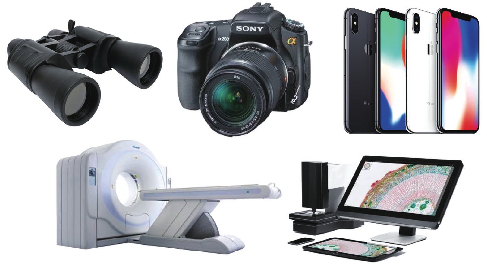
Fig. 1. Common optoelectronic imaging systems

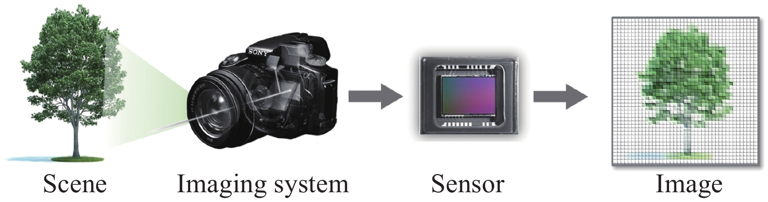
Fig. 2. Conventional optical imaging process

Fig. 3. Five goals for the development of optical imaging technology

Fig. 4. Conventional digital imaging processing is only a post-processing step in the whole imaging process

Fig. 5. Computational optical imaging process

Fig. 6. The revised discipline code of the National Natural Science Foundation of China in 2017. “Computational imaging” has been listed as an independent sub-direction of Information Science (F050109)

Fig. 7. Camera obscura box, 16^th century

Fig. 8. The Camera Obscura box used by Joseph Nicephore Niépce and his photo “the man with a horse”

Fig. 9. “Window at Le Gras” taken by Joseph Nicephore Niépce

Fig. 10. “Boulevard du Temple” taken by Joseph Nicephore Niépce, 1838

Fig. 11. William Henry Fox Talbot – An oak tree in winter (Negative and positive)

Fig. 12. Wet-collidion process

Fig. 13. Eadweard Muybridge——The horse in motion, 1878

Fig. 14. Brownie and Leica camera

Fig. 15. The advertisement of Kodak camera in New York, 1888.

Fig. 16. Thomas Sutton — Tartan Ribbon

Fig. 17. Kodachrome K135-20 Color Film

Fig. 18. Kodak instamatic camera

Fig. 19. The first of Ampex's videotape recorder VR-1000

Fig. 20. The first CCD camera developed by Boyle and Smith

Fig. 21. The first digital camera developed by Steven Sasson

Fig. 22. Mavica camera developed by SONY

Fig. 23. The first handphone with camera, J-SH04, developed by SHARP and J-Phone

Fig. 24. Nokia N90 handphone with Carl Zeiss optics

Fig. 25. Nikon SLR camera D1

Fig. 26. Apple iPhone 1 released in the Macworld 2007 by Steve Jobs

Fig. 27. Apple iPhone 4 released by Steve Jobs in 2010

Fig. 28. The first dual camera mobile phone — LG Optimus 3 D

Fig. 29. Structured light 3D face recognition technique in iPhone X

Fig. 30. Huawei P30 Pro and captured moon with highly clear surface details (though it is controversial that it is the result of AI synthesis)

Fig. 31. Comparison of film camera (Nikon F80) with digital camera (Nikon D50)

Fig. 32. Synthetic Aperture Radar (SAR), the earliest computational imaging technique

Fig. 33. Wave-front coding, the earliest optical imaging system involving the idea of computational imaging

Fig. 34. Basic configurations of the 3LCD projector and the DLP projector

Fig. 35. Sixteen photographs of a church taken at 1-stop increments from 30 to 1/1000 second^[23]

Fig. 36. Image dehazing using two images with orthogonal polarization state^[27]

Fig. 37. Program of Symposium on Computational Photography and Video in MIT, 2005 ^[29]

Fig. 38. The first light field camera developed by Ng and its commercialized verison——Lytro

Fig. 39. The 1st single-pixel camera developed by Rice University in 2006^[40-41]

Fig. 40. Principle of the GS phase retrieval method^[54-55]

Fig. 41. Principle of the Fourier transform profilometry method^[64]

Fig. 42. Principle of the conventional holographic imaging technique

Fig. 43. Principle of the off-axis digital holographic reconstruction

Fig. 44. Principle of coded aperture imaging and a photograph of a coded mask

Fig. 45. Topic categories of the Optica (formerly OSA) topic meeting COSI

Fig. 46. Professor Levoy's Google Pixel camera tops DXOMark several times

Fig. 47. "Computational imaging", "computational optics" and "computational photography" have gradually become marketing terms for smartphone manufacturers

Fig. 48. Facebook founder Mark Zuckerberg announced the renaming of Facebook as Meta and proposed the concept of "Metaverse", 3D sensing technology that promises to "digitize" the physical world and has great practical significance for the infrastructure and completion of Metaverse

Fig. 49. Classification of typical computational imaging techniques according to their ''objectives and motivations''

Fig. 50. Classification of the phase imaging techniques

Fig. 51. Zernike phase contrast microscopy and Differential Interference Contrast (DIC) microscopy

Fig. 52. Giant Michelson interferometer——LIGO wavefront detector

Fig. 53. Schematics of Shack-Hartmann and pyramid wavefront sensors

Fig. 54. Schematics of iterative phase retrieval techniques

Fig. 55. Schematic of Fourier ptychographic microscopy

Fig. 56. The wave-like pattern at the bottom of a swimming pool in sunlight. (The pool surface refracts the incident sunlight to produces the characteristic pattern)

Fig. 57. Applications of TIE in different research fields

Fig. 58. Generalized transport of intensity equation (GTIE) for partially coherent field

Fig. 59. Quantitative phase 3D imaging of a breast cancer cell using TIE^[238]

Fig. 60. Schematic diagram of the principle of quantitative phase imaging with DPC based on weak phase approximation

Fig. 61. Comparison illumination-optimized schemes. (a) PTFs and their synthetic PTFs corresponding to different illumination functions; (b) Isotropic quantitative phase imaging results under optimal illumination

Fig. 62. Imaging efficiency optimization schemes of DPC. (a) Triple-wavelength multiplexed illumination scheme; (b) Triple-wavelength illumination scheme for multimodal imaging and DPC; (c) Single-shot optimal illumination scheme of DPC

Fig. 63. Gradual increase in spectral imaging resolution

Fig. 64. The projection of the data cube in CTIS

Fig. 65. Schematic diagram of frame-type computer tomographic imaging spectrometer

Fig. 66. Single Disperser CASSI instrument designed by Wagadarikar, and the imaging results^[49]

Fig. 67. Schematic diagram of Fourier transform spectrometer

Fig. 68. Schematic diagram of Hadamard transform spectrometer

Fig. 69. Visible light, long wave infrared and polarization imaging results for the same scene

Fig. 70. Polarization imaging system based on rotating polarizer

Fig. 71. Split amplitude polarization imaging system developed by Farlow et al.^[299]

Fig. 72. Split aperture polarization imaging system

Fig. 73. Split focal plane polarization imaging system

Fig. 74. Structure diagram of multi-wavelength dual-rotating phase plate polarization imaging system designed by Luna et al.^[303]

Fig. 75. Atmospheric scattering model and comparison of images before and after polarization defogging

Fig. 76. PS-OCT imaging results of bovine myocardial samples. (a) 3D global structure map; (b) Local optical axis diagram; (c) Local delay map; (d) Local bi-direction attenuation map

Fig. 77. Six-step phase-shifting color photoelastic images of the diametric compression disk

Fig. 78. Representative techniques for 3D optical sensing

Fig. 79. (a) Schematic diagrams of stereo vision^[386]; (b) Time-of-flight method^[387]; (c) Laser scanning^[388];(d) Defocus recovery method^[389]

Fig. 80. Schematic diagram of fringe projection profilometry ^[403]

Fig. 81. Fringe order ambiguity in the wrapping phase of isolated objects and discontinuity surfaces^[424]

Fig. 82. Quad-camera real-time 3D measurement system based on stereo phase unwrapping and its measurement results. (a) Quad-camera real-time system proposed by our research group^[450]; (b) The real-time color 3D data in the dynamic scene obtained by our system^[451]; (c) The omnidirectional point cloud data obtained by our system^[456]; (d) 360° 3D surface defect detection obtained by our system^[457]

Fig. 83. Commercial products based on speckle correlation. (a) Kinect; (b) PrimeSense; (c) iPhone X

Fig. 84. Flowchart of the single-frame phase retrieval approach using deep learning and the 3D reconstruction results of different approaches. (a) The principle of deep-learning-based phase retrieval method^[460]; (b) Comparison of the 3D reconstructions of different fringe analysis approaches (FT, WFT, the deep-learning-based method, and 12-step phase-shifting profilometry) ^[460]; (c) The measurement results of a desk fan rotating at different speeds using our deep-learning method^[462]; (d) The dynamic 3D measurement result of a rotating workpiece by deep-learning-based color FPP method^[464]; (e) The dynamic 3D measurement result of a rotating bow girl model by composite fringe projection deep learning profilometry(CDLP)^[465]

Fig. 85. Various light field cameras based on microlens array

Fig. 86. Light field capture based on camera arrays. (a) Stanford Spherical Gantry^[479]; (b) Stanford large camera arrays^[481]; (c) Acquiring micro-object images with the 5×5 camera array system^[482]

Fig. 87. Computational light field. (a) Mask enhanced camera^[483]; (b) Compressive light field photography^[484]

Fig. 88. Light field imaging based on programmable aperture. (a) Programmable aperture light field camera^[485]; (b) Programmable aperture microscope^[251]

Fig. 89. Light field imaging in computational photography. (a) Light field refocusing^[476]; (b) Synthetic aperture imaging^[492]

Fig. 90. X-ray computed tomography. (a) 2D X-ray image versus; (b) 3D X-ray CT and Spiral cone beam scanning CT

Fig. 91. Typical brain MRI images

Fig. 92. Schematic of widefield (left) and confocal fluorescence microscope (right) optical path structure^[502]

Fig. 93. An example of the acquired 3 D image of a cell, captured by a fluorescence microscope

Fig. 94. x-y and x-z slice images of three-dimensional PSF are calculated theoretically. (a) x-y slice images. The number above each slice represent the distance between the slice along the z-axis direction and the central highlights of the point spread function; (b) x-z slice images. The number above each slice indicates the distance between the slice along the y-axis and the highlight of the point spread function center.

Fig. 95. Workflow of deconvolution three-dimensional fluorescence microscopic imaging

Fig. 96. Model of Light field microscope^[516]. (a) Traditional bright field microscope; (b) Light field microscopy^[516]; (c) Light field microscopic based on wave optics theory^[518]; (d) Fourier light field microscopy^[519]

Fig. 97. Light field applications in biological science. (a) Mouse with a head-mounted MiniLFM ^[522]; (b) Imaging Golgi-derived membrane vesicles in living COS-7 cells using HR-LFM ^[523]; (c) Migrasome dynamics during neutrophil migration in mouse liver with DAOSLIMIT^[525]; (d) Confocal light field microscopy, tracking and imaging whole-brain neural activity during larval zebrafish’s prey capture behavior and imaging and tracking of circulating blood cells in awake mouse brain^[524]

Fig. 98. Representative work on holographic diffraction tomography microscopy. （a） Rotating object measurements by Charriere et al^[532]; （b） Scanning galvanometer measurements by Choi et al^[534]; （c） Wedge prism scanning by Cotte et al^[537]; （d） Park's team^[547] for DMD scanning measurements

Fig. 99. Representative work on phase retrieval diffraction tomography microscopy. （a） Microscope platform rotating object measurements by Barty et al^[539] from the X diffraction imaging research team at the University of Melbourne, Australia; （b） Lens-free on-chip chromatography platform by the Ozcan group at UCLA^[548]; （c） Lens-free LED array-based platform by our group^[239]; （d） LED array-based microscopy platform of our group^[240]

Fig. 100. Two implementations of optical intensity diffraction tomography. (a) TIDT microscopy based on axial scanning; (b) FPDT microscopy based on illumination angle scanning

Fig. 101. Representative work on TIDT. （a） Quantitative phase imaging based on high numerical aperture ring illumination by our group^[238]; （b） TIDT with electronically controlled zoom lens by Alieva's group^[549] at the University of Madrid, Spain; （c） Multi-aperture optical intensity transfer diffraction tomography based on ring illumination by our group^[241]

Fig. 102. Representative work on FPDT. （a） FPDT 3D imaging based on a multilayer model by Waller's group at UC Berkeley^[550]; （b） FPDT without dark field intensity under the first-order Born approximation by Yang's group at Caltech^[185]; （c） FPDT with dark field intensity under the first-order Rytov approximation by our group^[186]

Fig. 103. Coherent measurement using interferometer. (a) Young’s interferometer^[561]; (b) Reversed-wavefront Young interferometer^[562]; (c) Non-redundant array^[563]; (d) Self-referencing interferometer^[565]; (e) Two-point interferometer; (f) Sagnac interferometer^[565-566]

Fig. 104. The principal and optical setup of phase-space tomography. (a) Principle of phase space tomography; (b) A pair of cylindrical lenses oriented perpendicularly are used to introduce astigmatism to the measurement. Intensities are measured at planes with axial coordinate z₀

Fig. 105. The direct measurement of phase space. (a) Direct measurement based on pinhole scanning^[569]; (b) Direct measurement based on microlens array^[570]

Fig. 106. The influence of two kinds of imaging resolution on the final image definition. (a) ideal high resolution image; (b) for the guidance system with small field of view, the resolution of the imaging system is finally determined by the optical resolution, that is, the aperture of the imaging system (as shown in Figure(c)), while for most search / tracking systems with wide field of view, the resolution of the imaging system is finally determined by the image resolution, that is, the pixel size of the detector (as shown in Figure(d))

Fig. 107. Diffraction resolution limit limited by the aperture of optical system (Airy spot). (a) The minimum resolvable distance (optical angular resolution) of the imaging system is inversely proportional to the aperture of the imaging system; (b)-(d) Airy spot images of two incoherent point targets at different distances

Fig. 108. Nyquist sampling limit limited by detector pixel size (mosaic effect). (a) Information aliasing caused by insufficient pixel sampling (excessive pixel size); (b) When the Nyquist sampling limit is exactly met; (c) The imaging effect of a typical infrared thermal imager for human targets at different distances (Pixel size: 38 μm. 320× 240 pixels, 50 mm focal length lens)

Fig. 109. Basic principle of pixel super-resolution reconstruction (Optimal solution of inverse ill-posed problem)

Fig. 110. Single frame reconstruction algorithm based on SCRNN

Fig. 111. Basic principle of passive subpixel moving super-resolution imaging

Fig. 112. Pixel level light intensity change caused by controllable sub-pixel movement

Fig. 113. Micro scanning device. (a) Optical refraction method; (b) Plate rotation method; (c) Piezoelectric ceramics body

Fig. 114. Changchun University of technology realizes sub-pixel light intensity conversion by using micro scanning imaging devices to realize image super-resolution^[589]

Fig. 115. Basic principle of coded aperture super resolution imaging^[594]

Fig. 116. (a) Visible coded aperture imaging system and its reconstruction results; (b) Infrared coded aperture imaging system and its reconstruction results

Fig. 117. Schematic diagram of Synthetic aperture radar

Fig. 118. (a) Principle diagram of laser synthetic aperture radar imaging based on optical fibers developed by Aerospace Corporation of the United States; (b) Comparison of imaging results (right image is diffraction-limited imaging results, left image is synthetic aperture results)

Fig. 119. Schematic of non-interferometric synthetic aperture imaging technology based on Fourier ptychography

Fig. 120. Reflective Fourier ptychography imaging system and schematic diagram^[600]

Fig. 121. Conventional incoherent synthetic aperture structure. (a) Michelson interferometer; (b) Common secondary structure; (c) Phased array structure

Fig. 122. Design model of the initial generation of SPIDER imaging conceptual system. (a) Design model and explosive view of SPIDER; (b) PIC schematics of the two physical baselines and three spectral bands; (c) Arrangement of SPIDER lenslets; (d) Corresponding spatial frequency coverage

Fig. 123. Incoherent synthetic aperture based on FINCH^[605]

Fig. 124. Super-resolution schematic diagram and result diagram of STORM^[608,615]

Fig. 125. The schematic diagram and results of super-resolution STED ^[618]

Fig. 126. The of SIM and the super-resolution reconstruction results of dynamic microtubules at different times ^[610]

Fig. 127. 3D super-resolution microscopy experimential results. (a) 3D SIM^[629]; (c) 3D STORM^[628]

Fig. 128. Two representative active ultrafast optical imaging techniques. (a) An ultrafast imaging technique based on sequential time all-optical mapping photography (STAMP) proposed by Nakagawa et al.^[647]; (b) An ultrafast imaging technique based on frequency recognition algorithm for multiple exposures (FRAME) proposed by Kristensson et al.^[649]

Fig. 129. A single-shot compressed ultrafast photography technique (CUP) proposed by Gao et al.^[653]

Fig. 130. Basic structure of a digital projector based on Digital Light Processing (DLP) technology and its core component DMD

Fig. 131. Working principle of a single DMD micromirror

Fig. 132. Binary time pulse width modulation mechanism for 8-bit grayscale image displayed by DMD

Fig. 133. The measurement result of beating rabbit heart^[671]

Fig. 134. 3D measurement and tracking a bullet fired from a toy gun^[669]. (a) Representative camera images at different time points; (b) Corresponding color-coded 3D reconstructions; (c) 3D reconstruction of the muzzle region (corresponding to the boxed region shown in (b)) as well as the bullet at three different points of time over the course of flight (7.5 ms, 12.6 ms, and 17.7 ms) (The insets show the horizontal (x–z) and vertical (y-z) profiles crossing the body center of the flying bullet at 17.7 ms); (d) 3D point cloud of the scene at the last moment (135 ms), with the colored line showing the 130 ms long bullet trajectory (The inset plots the bullet velocity as a function of time)

Fig. 135. Array projection technology and GOBO projection technology^[678-679]. (a) Array projector and three-dimensional measuring system set up with the projector; (b) GOBO projector and three-dimensional measuring system set up with the projector

Fig. 136. 3D reconstruction results for the airbag ejection process^[679]

Fig. 137. The systems and results of 5D hyperspectral imaging and high speed thermal imaging^[680-681]. (a) 5D hyperspectral imaging system; (b) High speed thermal imaging system; (c) 5D hyperspectral imaging results: The measurement of water absorption by a citrus plant; (d) High-speed thermal imaging results: The measurement of a basketball player at different times

Fig. 138. Measurement of a dynamic scene that includes a static model and a falling table tennis^[682], which are also not present in the training process. The first line to the third line pass µDLP obtains the corresponding 3D reconstruction of the fan at 1000 ~ 5000 r/min

Fig. 139. Working principle and imaging diagram of image intensifier

Fig. 140. EMCCD imaging result is compared with the reconstruction results of four different single photon algorithms in the case of long-distance imaging

Fig. 141. Principle of the photon counting imaging system

Fig. 142. Schematic diagram of echo and reconstruction results under different conditions

Fig. 143. Super-resolution results of target located at 8.2 km

Fig. 144. Illustration of long range single photon Lidar imaging

Fig. 145. Calculate the first photon 3D reconstruction of reflectance. (a)-(c) Point-by-point maximum likelihood processing in the three directions of the single photon result; (d)-(f) Corresponding reflectance estimation results; (g)-(i) Environmental noise processing; (j)-(l) 3D estimation results

Fig. 146. Illustration of the long-range active imaging over 201.5 km. Satellite image of the experiment implemented near the city of Urumqi, China, where the single-photon lidar is placed at a temporary laboratory in the wild. (a) Visible-band photograph of the mountains taken by a standard astronomical camera equipped with a telescope. The elevation is approximately 4500 m; (b) Schematic diagram of the experimental setup; (c) Photograph of the setup hardware, including the optical system (top and bottom left) and the electronic control system (bottom right; (d) View of the temporary laboratory at an altitude of 1770 m

Fig. 147. Reconstruction results of a scene over 201.5 km. (a) Real visible-band photo; (b) The reconstructed depth result by Lindell et al. in 2018 for the data with SBR ~ 0.04 and mean signal PPP ~ 3.58; (c) A 3 D profile of the reconstructed result

Fig. 148. Results of extremely weak light imaging based on deep learning. (a) Camera output with ISO 8000; (b) Camera output with ISO 409600; (c) Our result from the raw data of (a) ^[705]

Fig. 149. Diagram of proposed multi-scale network for single-photon 3D imaging with multiple returns

Fig. 150. The reconstruction results for three long range outdoor scenes. First row: A tall building, that locates at 21.6 km away from imaging system with a spatial resolution of 256×256, signal-to-noise ratio is 0.114, and 1.228 photons per pixel. Second row: That locates at 1.2 km away from our imaging system with a spatial resolution of 176×176, signal-to-noise ratio is 0.109, and 3.957 photons per pixel. Third row: A tall tower named Pole, that locates at 3.8 km away from our imaging system with a spatial resolution of 512×512, signal-to-noise ratio is 0.336, and 1.371 photons per pixel. GT denotes the ground truth depth maps captured by system with a long acquisition time

Fig. 151. For traditional optical systems, the two parameters of field of view and resolution are contradictory and cannot be taken into account at the same time. (a) The corresponding field of view angle of 35 mm SLR camera under different focal length; (b) Typical images taken by 35 mm SLR camera under different focal lengths

Fig. 152. GigaPan panoramic shooting system and pixel panorama obtained by shooting splicing

Fig. 153. ARGUS-IS system and its imaging effect. (a) ARGUS-IS system appearance; (b) The system uses 368 image sensors and four main lenses, of which 92 sensors are a group and share a main lens. By skillfully setting the installation position of sensors, the images obtained by each group of sensors are misaligned and complementary to each other, and then through image mosaic, better overall imaging results can be obtained; (c) The imaging system effectively covers 7.2 km × 7.2 km ground area at an altitude of 6 km

Fig. 154. Multi camera splicing system. (a) Light field acquisition system Immerge developed by lytro company; (b) Stanford semi ring camera array system; (c) Stanford planar camera array system; (d) Camatrix ring camera array system; (e) Tsinghua University birdcage camera array system

Fig. 155. (a) The research team of the Federal Institute of Technology (EPFL) in Lausanne, Switzerland, designed and developed the bionic compound eye imaging device Panoptic; (b) OMNI-R system with large field of view and high resolution; (c) Everyscope, avery ground-based telescope system developed by Nicholas Law

Fig. 156. Multiscale imaging system. (a) AWARE-2 structure drawing; (b) AWARE-10 structural drawing; (c) AWARE-40 structure drawing

Fig. 157. There is a tradeoff between the resolution and FOV in traditional microscopes: The FOV under low-magnification objective is large with the low resolution; for high-magnification objective, the resolution is improved while the FOV is reduced dramatically

Fig. 158. Four types of possible solutions to overcome the limited spatial bandwidth area of conventional microscopes. (a) On-chip lens-free holographic microscopy; (b) Fourier ptychography microscopy; (c) Synthetic aperture/FOV holographic microscopy; (d) Flow cytometric microscopy

Fig. 159. Sub-pixel super-resolution technology based on the lens-free holographic microscope. (a) Sub-pixel micro-scanning by moving illumination; (b) Active sub-pixel micro-scanning scheme with inclined parallel plate proposed by our research group

Fig. 160. Propagation phasor approach improves the data efficiency of holographic imaging^[750]

Fig. 161. High throughput quantitative microscopic imaging based on single frame Fourier ptychographic microscopy

Fig. 162. Schematic of single-pixel imaging^[803]

Fig. 163. Experimental set-up of two-dimension Fourier single-pixel imaging^[815]

Fig. 164. Experimental results of two-dimension Fourier single-pixel imaging^[815], the pixels of the reconstructed image are 256×256

Fig. 165. Experimental set-up of a stereo vision based 3D single-pixel imaging^[42]

Fig. 166. Overview of the image cube method^[824]. (a) The illuminating laser pulses back-scattered from a scene are measured as (b) broadened signals; (c) An image cube, containing images at different depths, is obtained using the measured signals; (d) Each transverse location has an intensity distribution along the longitudinal axis, indicating depth information; (e) Reflectivity and (f) a depth map can be estimated from the image cube, and then be used to reconstruct; (g) A 3D image of the scene

Fig. 167. Experimental results of multi-modality Fourier single-pixel imaging^[832]. (a) Fourier transform with spatial, 3D, and color three modality information of target object, where sampling ratio = 12%; (b) Image reconstructed from (a) with partial enlargement; (c)-(e) Top, perspective, and side views of the three-dimensional reconstruction of the object

Fig. 168. Experimental set-up of terahertz imaging with a single-pixel detector^[833]

Fig. 169. (a) Experimental setup^[833-835] for lens-free shadow imaging platform; (b) Cross-sectional scheme of the opToFluidic microscopy; (c) The top view of the device (b) The white circles are apertures. The gray dashed grid is the CMOS sensor coated with Al, and the blue lines are the whole microfluidic channel^[758,836]

Fig. 170. Schematic diagram of the lens-free on-chip fluorescent imaging platform, whose platform has unit magnification. The TIR occurs at the glass-air interface at the bottom facet of the cover glass. To avoid detection of scattered photons a plastic absorption filter is used behind the faceplate. （TIR: Short for total reflection; The image was modified from the references[837-839,841]）

Fig. 171. (a) Photograph of the lens-free tomography platform^[239]; (b) (Left) Photograph and (right) computer graphic diagram of a compact device for in situ nanolens formation and lens-free imaging^[847]

Fig. 172. 3D tomographic reconstructions of lens-free on-chip microscope based on multi-angle illumination. (a) The recovered refractive index depth sections of a slice of the uterus of Parascaris equorum; (b) The 3D renderings of the refractive index for the boxed area in (a)^[239]; (c) A tomogram for the entire worm corresponding to a plane that is 3 μm above the center of the worm; (d1)-(d2) y-z ortho slices from the anterior and posterior regions of the worm, respectively; (e1)-(e2) x-z ortho slices along the direction of the solid and dashed arrow in (c), respectively^[548]

Fig. 173. Incoherent lens-free imaging. (a) Two LEDs and (b) two one-dime coins separated by a distance of 15 mm by LI-COACH^[851]

Fig. 174. Lens-free imaging with FZP and incoherent illumination. (a) Real-time image capturing and reconstruction demonstration of a prototyped lens-free camera^[853]; (b) the reconstructions for the binary, grayscale and color images using the FZP single-shot lens-free camera^[856]

Fig. 175. FlatCam architecture. (a) A binary, coded mask is placed 0.5 mm away from an off-the-shelf digital image sensor; (b) An example of sensor measurements and the image reconstructed by solving a computational inverse problem

Fig. 176. Imaging principle of the system based on adaptive optics

Fig. 177. Low orbit satellite imaging by SOR telescope^[875]. (a) Uncompensated; (b) Compensated; (c) Compensated + image processing

Fig. 178. Basic layout of an adaptive optics system for imaging and vision testing

Fig. 179. Layered high resolution images taken by the AO-CSLO system. (a) Layer of human retina photoreceptors in vivo; (b) Layer of blood capillaries; (c) Layer of nerve fibers

Fig. 180. Application of adaptive optics in wide field fluorescence and confocal microscope

Fig. 181. Application of adaptive optics in confocal microscope and multiphoton microscope

Fig. 182. Application of adaptive optics in wide field fluorescence microscopy and super-resolution fluorescence microscopy. (a) Wide-field fluorescence microscopy of tubulin stained HeLa cells before(left) and after(right) correction^[892]; (b) A cluster of fluorescent microspheres of nominal diameter 121 nm, as imaged by conventional , confocal , and structured illumination microscopy^[894]; (c) By using DM and SLM to compensate all of the three path aberrations in STED microscopy^[897]; (d) Comparison of Confocal(left) and 3D STED(right) images of Atto647N labelled vesicular glutamate transporter in synaptic boutons in intact Drosophila brains^[895]

Fig. 183. Principle and experimental results of feedback-based wavefront shaping^[919]

Fig. 184. TM measurement principle based on scattering medium^[920]

Fig. 185. Optical phase conjugation based scattering imaging of biological tissue^[924]

Fig. 186. Schematic of the apparatus for non-invasive imaging through strongly scattering layers

Fig. 187. Single frame imaging based on speckle autocorrelation^[923] (a) Experimental set-up; (b) Raw camera image; (c) The autocorrelation of the seemingly information-less raw camera image; (d) The object’s image is obtained from the autocorrelation of by an iterative phase-retrieval algorithm; (e) Photograph of the experiment; (f) Raw camera image; (g)-(k) Left column: calculated autocorrelation of the image in (b), Middle column: reconstructed object from the image autocorrelation. Right column: image of the real hidden object

Fig. 188. Network schematic diagram of imaging through scattering medium based on deep learning^[927]

Fig. 189. Schematic diagram of typical non field of view imaging system

Fig. 190. (a) The capture process: capture a series of images by sequentially illuminating a single spot on the wall with a pulsed laser and recording an image of the dashed line segment on the wall with a streak camera; (b) An example of streak images sequentially collected. Intensities are normalized against a calibration signal. Red corresponds to the maximum, blue to the minimum intensities; (c) The 2D projected view of the 3D shape of the hidden object, as recovered by the reconstruction algorithm

Fig. 191. Dual photography of indirect light transmission^[934]. (a) System experimental device; (b) View of playing cards and books taken under indoor lighting; (c) Sample image obtained when the projector scans the indicated points on the playing cards in (d)

Fig. 192. Proposed secured single-pixel broadcast imaging system^[935]

Fig. 193. Diagram of confocal non-line-of-sight imaging

Fig. 194. Long-range NLOS imaging experiment. (a) An aerial schematic of the NLOS imaging experiment; (b) The optical setup of the NLOS imaging system, which consists of two synchronized telescopes for transmitter and receiver; (c) Schematic of the hidden scene in a room with a dimension size of 2 m×1 m; (d) An actual photograph of the NLOS imaging setup; (e)-(f) Zoomed-out and zoomed-in photographs of the hidden scene taken at location A, where only the visible wall can be seen; (g) Photograph of the hidden object, taken at the room located at B

Fig. 195. Comparison of the reconstructed results with different approaches. (a) The reconstructed results for the hidden scene of mannequin; (b) The reconstructed results for the hidden scene of letter H

Fig. 196. Nonuniformity of the thermal imaging camera caused by temperature jump of approximately 1 °C^[945]

Fig. 197. Scene-based non-uniformity correction results

Fig. 198. Non-uniformity correction method based om temporal high-pass filter

Fig. 199. The expected (mean) image of a long-time motion scene approximately satisfies the constant statistical assumption

Fig. 200. Experimental comparison plots of non-uniformity correction for various types of statistical constancy methods. (a) Uncorrected image; (b) Multiscale constant statistics; (c) Global constant statistics; (d) Local constant statistics

Fig. 201. Non-uniformity correction method based on neural network

Fig. 202. Motion compensation average method

Fig. 203. Nonuniformity correction method based on inter-frame registration

Fig. 204. Non-uniformity correction method based on inter-frame registration require accurate estimation of the relative displacement of an image pair imposed by strong non-uniformity

Fig. 205. In response to the problems of non-uniformity and low dynamic range of infrared detectors, Nanjing University of Science and Technology has developed high-performance infrared image signal processing technology, designed an ASIC with customized core algorithms based on scene-based non-uniformity correction and digital detail enhancement of infrared images, and developed a high-performance shutterless thermal imaging camera

Fig. 206. High-end optical instruments and their core technologies are the "bottle-neck" technologies and products embargoed by the Western military powers to China

Fig. 207. The Decree of the President of the People's Republic of China (No. 103) clearly states that under the condition that the function, quality and other indicators can meet the demand, the procurement of domestic scientific research instruments is encouraged

Table 1. Spatial bandwidth product of typical 35 mm SLR lens

Table 2. Spatial bandwidth product of typical microscopic objectives