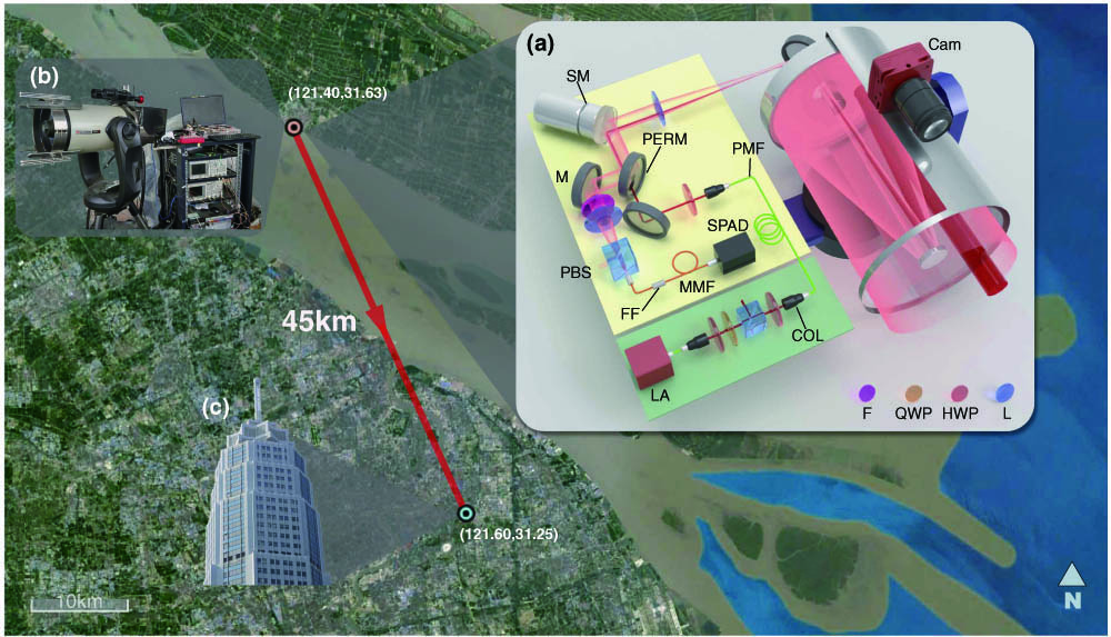
Fig. 1. Illustration of long-range active imaging. Satellite image of the experimental layout in Shanghai city, where the single-photon lidar is placed on Chongming Island and the target is a tall building in Pudong. (a) Schematic diagram of the setup. SM, scanning mirror; Cam, camera; M, mirror; PERM, 45° perforated mirror; PBS, polarization beam splitter; SPAD, single-photon avalanche diode; MMF, multimode fiber; PMF, polarization-maintaining fiber; LA, laser (1550 nm); COL, collimator; F, filter; FF, fiber filter; L, lens; HWP, half-wave plate; QWP, quarter-wave plate. (b) Photograph of the setup. The optical system consists of a telescope congregation and an optical-component box for shielding. (c) Close-up photograph of the target, the Pudong Civil Aviation Building. The building is 45 km from the single-photon lidar setup.

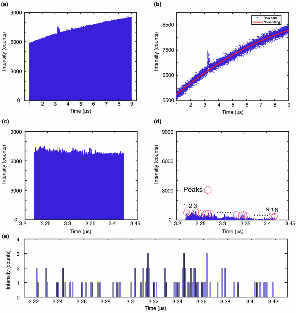
Fig. 2. Raw-data histogram and global-gating process. (a) Raw-data histogram for the 45 km imaging experiment over the laser period (∼10  μs). (b) Noise fitting for the background noise, which comes mainly from the internally reflected ASE noisy photons and increases with time following a binomial distribution. (c) Censored time bins for reconstructions. (d) Illustration of the signal counts. (e) Illustration of a histogram of a single pixel within the effective signal gate Tgate.

Fig. 3. Long-range 3D imaging over 45 km. (a) Real visible-band image (tailored) of the target taken with a standard astronomical camera. This photograph is substantially blurred due to the inadequate spatial resolution and the air turbulence in the urban environment. The red rectangle indicates the approximate lidar FoR. (b)–(e) Reconstruction results obtained by using the pixelwise maximum likelihood (ML) method, photon-efficient algorithm [18], unmixing algorithm by Rapp and Goyal [21], and the proposed algorithm, respectively. The single-photon lidar recorded an average PPP of ∼2.59, and the SBR was ∼0.03. The calculated relative depth for each individual pixel is given by the false color (see color scale on right). Our algorithm performs much better than the other state-of-the-art photon-efficient computational algorithms and provides sufficient resolution to clearly resolve the 0.6 m wide windows [see expanded view in inset of (e)].

Fig. 4. Long-range target taken in daylight over 21.6 km. (a) Topology of the experiment. (b) Ground-truth image of the target (building K11). (c) Visible-band image of the target taken with a standard astronomical camera. (d)–(g) Depth profile taken with the proposed single-photon lidar in daylight and reconstructed by applying the different algorithms to the data with 1.2 signal PPP and SBR=0.11. (d) Reconstruction with the pixelwise ML method. (e) Reconstruction with the photon-efficient algorithm [18]. (f) Reconstruction with the algorithm of Rapp and Goyal [21]. (g) Reconstruction with the proposed algorithm. The peak signal-to-noise ratio (PSNR) was calculated by comparing the reconstructed image with a high-quality image obtained with a large number of photons. The proposed method yields a much higher PSNR than the other algorithms.

Fig. 5. Long-range target at 21.6 km imaged in daylight and at night. (a) Visible-band image of the target taken with a standard astronomical camera. (b) Depth profile of image taken in daylight and reconstructed with signal PPP=1.2, SBR=0.11. (c) Depth profile of image taken at night and reconstructed with signal PPP=1.2, SBR=0.15.

Fig. 6. Reconstruction of multilayer depth profile of a complex scene. (a) Visible-band image of the target taken by a standard astronomical camera mounted on the imaging system with an f=700  mm camera lens. (b), (c) Depth profile taken by the proposed single-photon lidar over 2.1 km, and recovered by using the proposed computational algorithm. Trees at different depths and their fine features can be identified.

Table 1. Summary of Representative Single-Photon Imaging Experiments, Focusing on Imaging Distance and Sensitivity