Long-range active optical imaging has widespread applications, ranging from remote sensing [1–3], satellite-based global topography [4,5], and airborne surveillance [3], to target recognition and identification [6]. An increasing demand for these applications has resulted in the development of smaller, lighter, lower-power lidar systems, which can provide high-resolution three-dimensional (3D) imaging over long ranges with all-time capability. Time-correlated single-photon-counting (TCSPC) lidar is a candidate technology that has the potential to meet these challenging requirements [7]. Particularly, single-photon detectors [8] and arrays [9,10] can provide extraordinary single-photon sensitivity and better timing resolution than analog optical detectors [7]. Such high sensitivity allows lower-power laser sources to be used and can permit time-of-flight imaging over significantly longer ranges. Tremendous effort has thus been devoted to the development of single-photon lidar for long-range 3D imaging [11–14].

In long-range 3D imaging, a frontier question is the distance limit, i.e., over what distances can the imaging system work? For a single-photon lidar system, the echo light signal, and thus the signal-to-background ratio (SBR), decrease rapidly with imaging distance R, which imposes limits on the useful image reconstruction [15]. On hardware, the lidar system should possess both high efficiency for collecting the back-scattered photons and low background noise. On software, a computational algorithm with high photon efficiency is demanding [16]. Indeed, an important research trend today is the development of efficient algorithms for imaging with a small number of photons [17]. High-quality 3D structure and reflectivity by an active imager detecting only one photon per pixel (PPP) have been demonstrated, based on the approaches of pseudo-array [18,19], single-photon camera [20], unmixing signal/noise [21], and machine learning [22].

Our primary interest in this work is to significantly push the imaging range. Single-photon imaging up to the ten kilometers range has been reported in Ref. [23]. Very recently, super-resolution single-photon imaging over an 8.2 km range has also been demonstrated by us [24]. Nonetheless, before this work, the imaging range was limited to 10 km. Further extending the imaging range faces rather low photon counts and low signal-to-noise ratio, which casts challenge to both the imaging hardware and the reconstruction algorithm.

We approach the challenge of ultra-long-range imaging by developing advanced techniques based on both hardware and software implementations that are specifically designed for long-range scenarios. On the hardware side, we developed a high-efficiency coaxial-scanning system and optimized the system design to efficiently collect the few echo photons and suppress the background noise. On the software side, we developed a pre-processing approach to censor noise and a computational algorithm to reconstruct images with low-light data (i.e., ∼1 signal PPP) that are mixed with strong background noise (i.e., SBR∼1/30). These improvements allow us to demonstrate single-photon 3D imaging over a distance of 45 km in an urban environment. Moreover, by applying the microscanning approach [24,25], the demonstrated transverse resolution is about 0.6 m at the far field of 45 km.

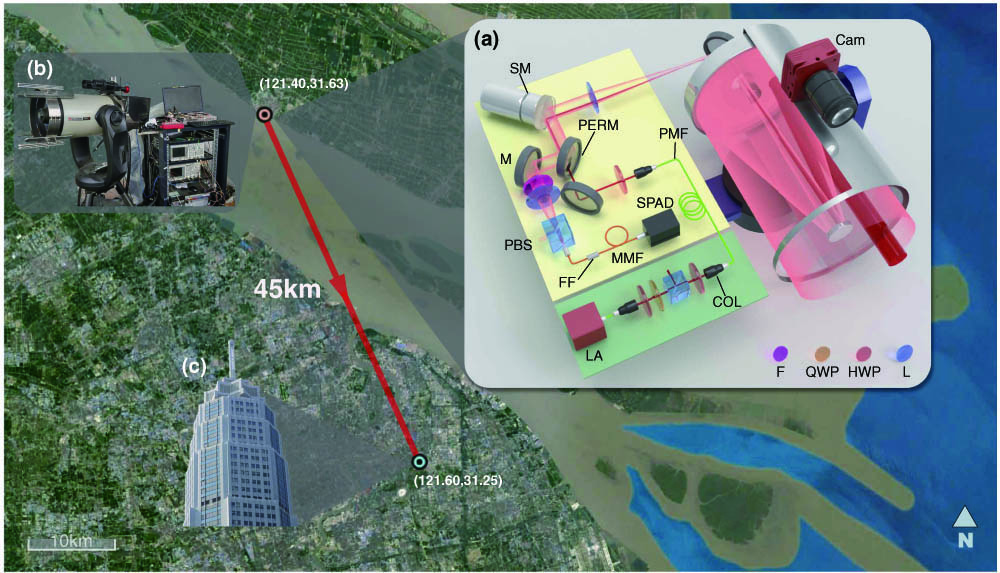
Figure 1 shows a bird’s eye view of the long-range active-imaging experiment, where the setup is placed at Chongming Island in Shanghai city, facing a target of a tall building located at Pudong across the river. The optical transceiver system incorporated a commercial Cassegrain telescope with a 280 mm aperture and a high-precision two-axis automatic rotating stage to allow large-scale scanning of the far-field target. The optical components were assembled on a custom-built aluminum platform integrated with the telescope tube. The entire optical hardware system is compact and suitable for mobile applications [see Fig. 1(b)].

Specifically, as shown in Fig. 1(a), an erbium-doped near-infrared fiber laser (1550.1±0.1nm, 500 ps pulse width, 100 kHz repetition rate) served as the light source for illumination. The maximal average laser power transmitted was 120 mW, which is equivalent to 1.2 μJ per pulse. There are several advantages of using a near-infrared wavelength, such as reduced solar background, low atmospheric absorption loss, and a higher eye safety threshold compared with the visible band. The laser output was coupled into the telescope through a small aperture consisting of a 45° oblique hole through the mirror. The echo light will fill the unobstructed part of the telescope and be transmitted to the mirror, where the size of the light spot is larger than the oblique hole aperture, which ensures that most of the echo light is reflected to the rear optical path for coupling.

The transmitting and receiving beams were coaxial, where the transmitting beam has a divergence angle of 35 μrad, and the receiving beam has a field of view (FoV) of 22.3 μrad. The returned photons were reflected by the perforated mirror and passed through two wavelength filters (1500 nm long-pass filter, 9 nm bandpass filter). Then, the returned photons were collected by a focal lens. A polarization beam splitter (PBS) coupled only the horizontal-polarization light into a multimode-fiber filter (1.3 nm bandpass). Finally, the photons were detected by an InGaAs/InP single-photon avalanche diode detector (SPAD) operated at free-running mode (15% detection efficiency) [26]. This means that our system does not have any prior information for the location/width of the returned signal’s time-gating window.

Detection events are time stamped with a homemade time-to-digital convertor (TDC) with 50 ps time jitter. The time jitter of the entire lidar system was measured at ∼1ns. It means that the system can obtain the depth measurement with an accuracy of 15 cm. In addition, a standard camera was paraxially mounted on the telescope to provide a convenient direction and alignment aid for long distances.

To achieve a high-efficiency, low-noise coaxial single-photon lidar, we implemented several optimized optical designs, most of which differed from previous single-photon lidar experiments [11–13,23]. With these new technologies, the imaging range can be greatly extended.

System.Xml.XmlElementSystem.Xml.XmlElementSystem.Xml.XmlElementSystem.Xml.XmlElementSystem.Xml.XmlElement

The long-range operation of the lidar system involves two challenges that limit useful image reconstruction. (i) Due to the divergence of the light beam, the receiver’s FoV, projected on the remote target, covers several reflectors with multiple returns [28–30], which deteriorates the resolution of the image. (ii) The extremely low SBR, together with multiple returns per pixel, limits the pixelwise-adaptive unmixing of signal from noise [21]. These two challenges were not considered in previous algorithms [16,18,19–22]. Recently, the issue of multiple returns has been addressed in different imaging scenarios, such as underwater imaging [30] and imaging through scattering media with multiple layers [31,32], most of which are aimed at scenes with partially transmissive objects. In contrast, we focused on the multiple-returns problem in a long-range situation caused by the divergence of the laser beam and the receiver’s large FoV, and proposed an approach to improve the resolution. We abstract the entire image reconstruction as a convolutional model instead of pixelwise processing and describe the reconstruction as an inverse deconvolution problem. To solve this problem, we modified the convex-optimization solver [33] to directly solve the 3D matrix. Rather than the previous two-step method that optimizes reflectivity and depth separately [16,18,19–21], our scheme uses a 3D spatiotemporal matrix to solve reflectivity and depth simultaneously. This can include the correlations between reflectivity and depth in the optimization. Also, it can avoid introducing the reflectivity reconstruction error into the depth estimation.

The forward model is based on Ref. [29], which describes the imaging condition through a thin diffuser. Here, we demonstrate this model more explicitly under long-range conditions. Suppose that the laser illuminates the scene at a scanning angle (θx, θy). Under long-range conditions, due to the divergence of the beam, a large light spot, illuminating on the scene, has a spatial 2D Gaussian distribution with kernel hxy. Due to the laser pulse width and detector jitter, the detected photons have a timing jitter, which is a temporal 1D Gaussian distribution with kernel ht. The detector rate function R(t;θx,θy) can be written as [29] for t∈[0,Tr), where Tr denotes the repetition period of the laser; [r(θx′,θy′), d(θx′,θy′)] is the [intensity, depth] pair for the scanning direction (θx′, θy′); FoV denotes the FoV of the detector; c is the speed of light; b describes background noise, and hxy and ht denote the spatial and temporal kernels, respectively.

We can discretize the continuous rate function in Eq. (1) into a 3D matrix with pixels and time bins. With nx×ny as the number of pixels, the scene can be described by a reflectivity matrix A and a depth matrix D(A,D∈Rnx×ny). Let Δ denote the bin width, where the detector records the photon-count histogram with nt=Tr/Δ bins. To transform the two matrices of A,D into one matrix, we construct a 3D (nx×ny×nt) matrix RD whose (i,j)-th pixel is a vector with only one nonzero entry. The value of this entry is Aij, and its index is Tij=round[2×Dij/(cΔ)]. To match this 3D formulation, let B be a (bΔ)-constant matrix of size nx×ny×nt, and let h be the outer product of hxy and ht, which is also a 3D matrix of size kx×ky×kt, denoting a spatiotemporal kernel.

According to the theory of photodetection in which the photon detection generated by the SPAD is an inhomogeneous Poisson processing, we obtain the distribution of our detected photon histogram matrix S of size nx×ny×nt: where * denotes the convolution operator. Next, our aim is to get the fine estimate of RD based on this probabilistic measurement model from the raw data S acquired from SPAD.

The reconstruction contains two parts: (i) a global gating approach to unmix signal from noise; (ii) an inverse 3D deconvolution based on the modified SPIRALTAP solver [33].

In our experiment, we operate the SPAD in free-running mode with an operation time of ∼10μs [see Fig. 2(a)], the same as the laser period. This can cover a wide range of blind depth measurements. We post-select the signals by following an automated global gating process to extract the time-tagged signals. Our global gating consists mainly of the following two processes. (i) Noise-fitting: different from the pixelwise gating [21], we sum the detection counts from all pixels and generate a total raw-data histogram, as shown in Fig. 2(a). The background noise consists of ambient light, dark counts, and the internally reflected ASE noise. In our experiment, the ASE noise is about 6000 counts/s, and the dark counts rate is about 2000 counts/s. As for the ambient light, it can be neglected at night. Therefore, the background noise comes mainly from the ASE noise. Note that the ASE noise arising from the pulsed laser increases over time within the laser period (∼10μs). In each pulse cycle, the photon population in the upper laser level gradually increases, and it suddenly drops after the pulse emitting out [34]. The ASE noise is correlated with the photon population, resulting in its increase over time. The exact relationship for ASE noise over time can be complex for different laser systems [34]. In our experiment, after careful calibrations, we find that the ASE noise can be well described using quadratic polynomial fitting, as shown in Fig. 2(b), where the relative standard deviation between the data and the fitting curve is less than 5%. (ii) Peak searching: we apply a peak-searching process to determine the position of the effective signal gate Tgate. For the duration of Tgate, we generally select a typical value of 200 ns (∼30m), which can cover the depths for most of natural targets. Note that for a multiple-layer scene, multiple effective signal gates will be selected. We censor the data out of its Tgate from the raw data and obtain the censored signal bins in Fig. 2(c). Also, we set a threshold (according to the noise-fitting results) for each signal time bin to further censor the noisy bins within Tgate.

Overall, the general procedure for global gating is listed in Algorithm 1. The stepwise descriptions of the procedure can be summarized as follows. (i) Form histograms H[T] and h[t] from the raw data with two different bin resolutions Tcoarse and Tfine; (ii) apply a quadratic function to fit h[t] and downsample this fit for H[T]; (iii) compute the deviations between each histogram and its respective fit; (iv) find the position of the peak in the coarse deviation data E1[t] and refine this position estimate with the fine deviation data E2[T]; (v) within the time interval containing the signal peak, retain only the bins (fine bins) above a data-dependent threshold (the error standard deviation). Note that the output of the global gating procedure indicates which bins are considered as signal and need to be included. Last, the output signal bins are used to censor the raw data by judging whether each photon arriving time is within these signal bins.

Figure 2(d) shows the rough signal photons for all the pixels within Tgate. Figure 2(e) shows the raw data of a single pixel within Tgate, where one of the highly reflective pixels is selected for the illustration of multiple peaks per pixel. Clearly, the issue of the multiple returns results in several peaks per pixel, which makes it difficult to perform the conventional pixelwise-adaptive gating [21].Algorithm 1.

Global gating.

For the censored signal bins in Fig. 2(c), we solve an inverse optimization problem to estimate RD. Let LRD(RD;S,h,B) denote the negative log-likelihood function of the RD derived from Eq. (2). Then the deconvolution problem is described by where the constraint RDi,j,k≥0 comes from the nonnegativity of reflectivity. Both the negative Poisson log-likelihood cost function LRD and the non-negativity constraint of the RD are convex; thus, the global minimizer could be found by a global optimization.

A widely used solver is SPIRALTAP, as demonstrated previously in Refs. [16,18,20,21]. Nonetheless, the existing SPIRALTAP solver cannot be applied directly to solve Eq. (3), because all the operators and matrices in our forward model are represented in the 3D spatiotemporal domain, whereas the existing SPIRALTAP can solve only optimization problems represented in the 2D domain [16,18,20,21]. Consequently, we generalize the existing SPIRALTAP to a 3D form by analogy. For this purpose, we applied a blurring matrix h, denoting the spatiotemporal kernel. h has dimensions of kx×ky×kt, and its elements are the product of the spatial (transversal) distribution and temporal (longitudinal) distribution for pixel (i,j). In implementation, the size of h is related to the FoV of the receiver and the system jitter. For more details about h, one can refer to the processing code available online [35].

We present an in-depth study of our imaging system and algorithm for a variety of targets with different spatial distributions and structures over different ranges [35]. The experiments were done in an urban environment in Shanghai. In experiment, we perform blind lidar measurements without any prior information for the time location of returned signals. Depth maps of the targets were reconstructed by using the proposed algorithm with ∼1PPP for signal photons and an SBR as low as 0.03. Here, we define the SBR as the signal detection counts (i.e., the back-reflections from the target) divided by the noise detection counts (i.e., the ambient light, dark counts, and ASE noise) within the 200 ns timing gate after the global gating process (see Section 2.A). We also made accurate laser-ranging measurements to determine the absolute distance to the targets; the laser pulses of three different repetition rates were employed to extend the unambiguous range [36].

We first show the imaging results for a long-range target, called the Pudong Civil Aviation Building, at a one-way distance of about 45 km. Figure 1 shows the topology of the experiment. The imaging setup was placed on the 20th floor of a building, and the target was on the opposite shore of the river. The ground truth of the target is shown in Fig. 1(c). Figure 3(a) shows a visible-band photograph, taken with a standard astronomical camera (ASI120MC-S). This photograph was substantially blurred due to the inadequate spatial resolution and the air turbulence in the urban environment. We adopted our single-photon lidar to do the imaging at night and produce a (128×128)-pixel image. A modest laser power of 120 mW was used for the data acquisition. The averaged PPP was ∼2.59, and the SBR was 0.03. Note that these PPP and SBR were calculated based on all the pixels in the entire scene. If we consider only the pixels with valid surfaces, the averaged PPP and SBR are about 6.45 and 0.08, respectively. The plots in Figs. 3(b)–3(e) show the reconstructed depth obtained by using various imaging algorithms, including the pixelwise maximum likelihood (ML), photon-efficient algorithm by Shin et al. [18], unmixing algorithm by Rapp and Goyal [21], and the algorithm proposed herein. The proposed algorithm recovers the fine features of the building, allowing the scenes with multilayer distribution to be accurately identified. The other algorithms, however, fail in this regard. These results clearly demonstrate that the proposed algorithm operates better for spatial and depth reconstruction of long-range targets. Furthermore, we used the microscanning approach [24] by setting a fine interval scan (half FoV interval) to improve the resolution. The result reaches a spatial resolution of 0.6 m, which resolves the small windows of the target building [see inset in Fig. 3(e)].

To quantify the performance of the proposed technique, we show an example of a 3D image obtained in daylight of a solid target with complex structures at a one-way distance of 21.6 km [see Fig. 4(a)]. The target is part of a skyscraper called K11 [see Fig. 4(b)] that is located in the center of Shanghai city. Before data acquisition, a photograph of the target was taken with a visible-band camera [see Fig. 4(c)]; the resulting visible-band image is blurred because of the long object distance and the urban air turbulence. The single-photon lidar data were acquired by scanning 256×256 points at an acquisition time per point of 22 ms and with a laser power of 100 mW. The total acquisition time was about 25 min. We performed calculations according to our model in Section 3.A, where the difference between the expected photon number and the measured photon number is within an order of magnitude. For the entire scene, the average PPP was 1.20, and the SBR was 0.11. For the pixels with valid depths only, the average PPP was 1.76, and the SBR was 0.16. The plots in Figs. 4(d)–4(g) show the reconstructed depth profiles using different algorithms. The proposed algorithm allows us to clearly identify the shape of the grid structure on the walls and the symmetrical H-like structure at the top of the building. The quality of the reconstruction is quantified based on the peak signal-to-noise ratio (PSNR) by comparing the reconstructed image with a high-quality image obtained by using a large number of photons. The PSNR is evaluated for all the pixels in the entire scene, where the pixels without valid depths are set to zero. The PSNR of the proposed algorithm is 14 dB better than that of the ML method, and 8 dB better than that of the unmixing algorithm. In this reconstruction, we have chosen a particular regularizer (3D TV semi-norm) based on the characteristics of our target scenes [35].

To demonstrate the all-time capability of the proposed lidar system, we used it to image building K11 both in daylight and at night (i.e., 11:00 AM and 12:00 PM) on June 15, 2018, and compared the resulting reconstructions. The proposed single-photon lidar gave 1.2 signal PPP and an SBR of 0.11 (0.15) in daylight (at night). Figures 5(b) and 5(c) show front-view depth plots of the reconstructed scene. The single-photon lidar allows the surface features of the multilayer walls of the building to be clearly identified both in daylight and at night. The enlarged images in Figs. 5(b) and 5(c) show the detailed features of the window frames, although, due to increased air turbulence during the day, the daytime image is slightly blurred compared with the nighttime image.

Finally, Fig. 6 shows a more complex natural scene with multiple trees and buildings at a one-way distance of 2.1 km. This scene was selected and scanned in daytime to produce a (128×256)-pixel depth image. Figure 6(b) shows the depth profile of the scene, and Fig. 6(c) shows a depth-intensity plot. The conventional visible-band photograph in Fig. 6(a) is blurred mainly because of smog in Shanghai, and does not resolve the different layers of trees in the 2D image. In contrast, as shown in Figs. 6(b) and 6(c), the proposed lidar system clearly resolves the details of the scene, such as the fine features of the trees. More importantly, the 3D capability of the single-photon lidar system clearly resolves the multiple layers of trees and buildings [see Fig. 6(b)]. This result demonstrates the superior capability of the near-infrared single-photon lidar system to resolve targets through smog [37].

To summarize, we demonstrate active single-photon 3D imaging at ranges of up to 45 km; this beats the previous record of 10 km [23]. Table 1 shows more comparisons with previous experiments. The 3D images are generated at the single-photon per-pixel level, which allows for target recognition and identification at very low light levels. The proposed high-efficiency coaxial single-photon lidar system, noise-suppression method, and advanced computational algorithm open new opportunities for low-power lidar imaging over long ranges. These results could facilitate the adaptation of the system for use in future multibeam single-photon lidar systems with Geiger-mode SPAD arrays for rapid remote sensing [38]. Nonetheless, the SPAD arrays face the limitations of data readout and storage [9,10], which require future technical improvements. For instance, a high-speed circuitry and efficient readout strategies are needed to speed up the readout process [39]. Another limitation of SPAD arrays is the low fill factor caused by the additional in-pixel circuitry for TDC, which can be improved by using microlens arrays [39,40]. Moreover, the advanced detection techniques such as a superconducting nanowire single-photon detector (SNSPD) [8] can be used to improve the efficiency and decrease the noise, as demonstrated in other lidar systems [12,41,42]. Furthermore, our framework does not consider the turbulence effects in long-range imaging. Nonetheless, the turbulence effect can be included in our forward model and reconstruction, by modifying the integration domain and the distribution of spatial and temporal kernels in Eq. (1) according to the model of the turbulence effect. Finally, the imaging experiment we completed is through only the horizontal atmosphere. The lidar’s SNR will gain when the light passes the atmosphere vertically. In the future, low-power single-photon lidar mounted on LEO satellites, as a complement to traditional imaging, can provide high-resolution, richer 3D images for a variety of applications.

Acknowledgment. The authors acknowledge insightful discussions with Cheng Wu, Ting Zeng, and Qi Shen.