Author Affiliations
School of Optoelectronic Engineering, Changchun University of Science and Technology, Changchun, Jilin 130022, Chinashow less
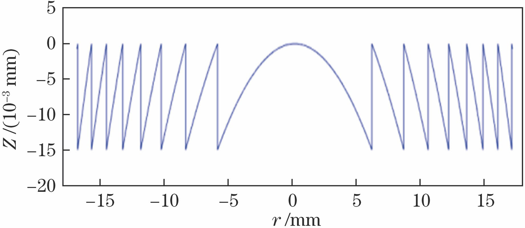
Fig. 1. Diffraction surface after magnification
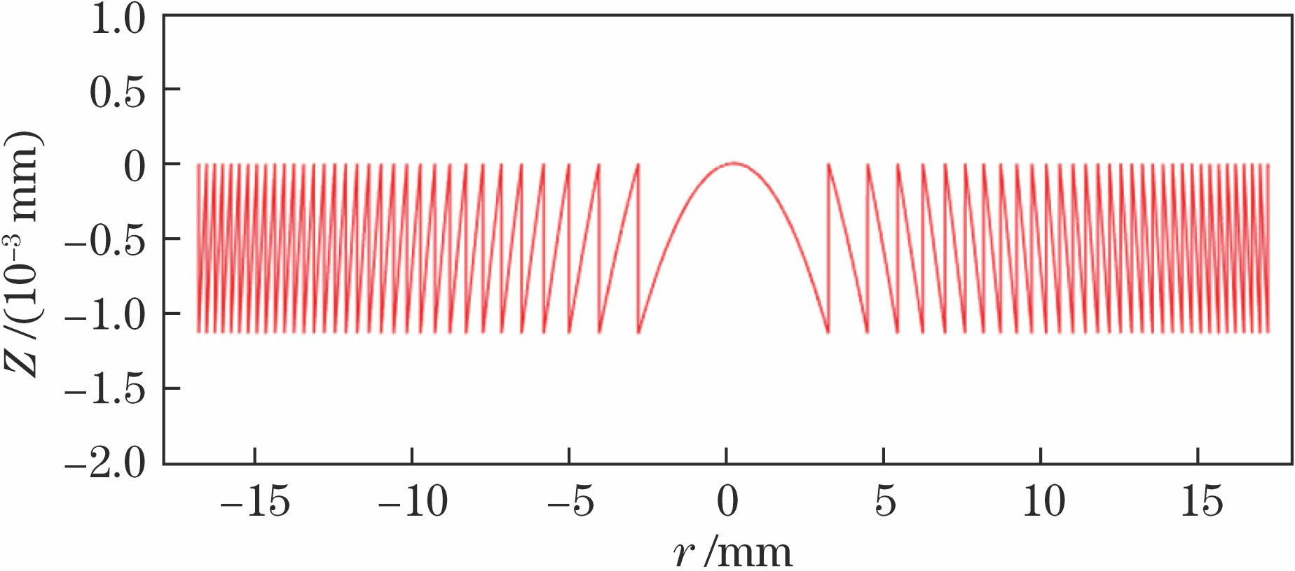
Fig. 2. Designed diffraction surface
Fig. 5. Main effect plot of mean of weighted evaluation values
Fig. 6. Simulation result by Moldflow
Fig. 7. Height error simulation results
Fig. 8. Period error simulation results
Fig. 9. Mold core machining error
Fig. 10. Microstructure period error curve
Fig. 11. Microstructure height error curve
Fig. 12. Mold core microstructure measurement results
Fig. 13. Lens measurement results without optimization
Fig. 14. Lens measurement results after optimization
Fig. 15. Lens measurement results after compensation
| Factor | Symbol | Level 1 | Level 2 | Level 3 |
|---|
| Melt temperature | A /℃ | 230 | 240 | 250 | | Mold temperature | B /℃ | 65 | 75 | 85 | | Injection time | C /s | 2 | 4 | 6 | | Cooling time | D /s | 40 | 60 | 80 | | Holding pressure | E /MPa | 120 | 135 | 150 | | Holding time | F /s | 15 | 25 | 35 |
|
Table 1. Control factors and factor levels of Taguchi experiment
| Run | A /℃ | B /℃ | C /s | D /s | E /MPa | F /s | ΔH /μm | fi1 | ΔT /μm | fi2 | Fi |
|---|
| 1 | 230 | 65 | 2 | 40 | 120 | 15 | 6.1 | -15.7066 | 59.1 | -35.4317 | -1.8954 | | 2 | 230 | 65 | 2 | 40 | 135 | 25 | 5.5 | -14.8073 | 53.1 | -34.5019 | -1.8198 | | 3 | 230 | 65 | 2 | 40 | 150 | 35 | 7.9 | -17.9525 | 86.5 | -38.7403 | -2.1137 | | 4 | 230 | 75 | 4 | 60 | 120 | 15 | 6.0 | -15.5630 | 62.3 | -35.8898 | -1.9015 | | 5 | 230 | 75 | 4 | 60 | 135 | 25 | 4.3 | -12.6694 | 38.7 | -31.7542 | -1.6241 | | 6 | 230 | 75 | 4 | 60 | 150 | 35 | 7.3 | -17.2665 | 79.0 | -37.9525 | -2.0537 | | 7 | 230 | 85 | 6 | 80 | 120 | 15 | 6.8 | -16.6502 | 80.1 | -38.0727 | -2.0246 | | 8 | 230 | 85 | 6 | 80 | 135 | 25 | 3.8 | -11.5957 | 20.2 | -26.1070 | -1.3978 | | 9 | 230 | 85 | 6 | 80 | 150 | 35 | 4.0 | -12.0412 | 24.0 | -27.6042 | -1.4663 | | 10 | 240 | 65 | 4 | 80 | 120 | 25 | 7.9 | -17.9525 | 86.8 | -38.7704 | -2.1946 | | 11 | 240 | 65 | 4 | 80 | 135 | 35 | 3.8 | -18.8897 | 89.8 | -39.0655 | -2.1731 | | 12 | 240 | 65 | 4 | 80 | 150 | 15 | 3.4 | -10.6296 | 32.6 | -30.2644 | -1.4713 | | 13 | 240 | 75 | 6 | 40 | 120 | 25 | 5.6 | -14.9638 | 49.0 | -33.8039 | -1.8072 | | 14 | 240 | 75 | 6 | 40 | 135 | 35 | 6.8 | -16.6502 | 71.5 | -37.0861 | -1.9950 | | 15 | 240 | 75 | 6 | 40 | 150 | 15 | 6.3 | -15.9868 | 62.1 | -35.8618 | -1.9232 | | 16 | 240 | 85 | 2 | 60 | 120 | 25 | 5.5 | -14.8073 | 52.5 | -34.4032 | -1.8169 | | 17 | 240 | 85 | 2 | 60 | 135 | 35 | 3.3 | -10.3703 | 16.3 | -24.9103 | -1.2969 | | 18 | 240 | 85 | 2 | 60 | 150 | 15 | 7.3 | -17.5012 | 84.2 | -38.5062 | -2.0828 | | 19 | 250 | 65 | 6 | 60 | 120 | 35 | 9.7 | -19.7354 | 104.4 | -40.3740 | -1.9972 | | 20 | 250 | 65 | 6 | 60 | 135 | 15 | 5.3 | -14.4855 | 53.2 | -34.5182 | -1.8033 | | 21 | 250 | 65 | 6 | 60 | 150 | 25 | 4.9 | -13.8039 | 46.6 | -33.3677 | -1.7326 | | 22 | 250 | 75 | 2 | 80 | 120 | 35 | 8.4 | -18.4856 | 92.3 | -39.3040 | -2.1589 | | 23 | 250 | 75 | 2 | 80 | 135 | 15 | 6.4 | -16.1236 | 75.3 | -37.5359 | -1.9806 | | 24 | 250 | 75 | 2 | 80 | 150 | 25 | 4.3 | -12.6694 | 15.3 | -23.6938 | -1.3823 | | 25 | 250 | 85 | 4 | 40 | 120 | 35 | 4.0 | -12.0412 | 25.0 | -27.9588 | -1.4770 | | 26 | 250 | 85 | 4 | 40 | 135 | 15 | 8.3 | -18.3816 | 88.2 | -38.9094 | -2.1415 | | 27 | 250 | 85 | 4 | 40 | 150 | 25 | 4.5 | -13.0643 | 31.6 | -29.9937 | -1.5922 |
|
Table 2. Orthogonal test data and signal-to-noise ratio for L27(36)
| Factor | G | S | M | L | P |
|---|
| A | 2 | 1.07 | 0.54 | 0.13 | 0.88 | | B | 2 | 7.98 | 3.99 | 1.00 | 0.39 | | C | 2 | 0.18 | 0.09 | 0.02 | 0.98 | | D | 2 | 0.11 | 0.05 | 0.01 | 0.99 | | E | 2 | 5.93 | 2.96 | 0.74 | 0.49 | | F | 2 | 11.34 | 5.67 | 1.42 | 0.28 | | Residuals | 14 | 55.96 | 3.99 | | | | Total | 26 | 82.55 | | | |
|
Table 3. ANOVA of signal-to-noise ratio for height error
| Factor | G | S | M | L | P |
|---|
| A | 2 | 101.80 | 50.90 | 0.06 | 0.94 | | B | 2 | 2065.30 | 1032.65 | 1.23 | 0.32 | | C | 2 | 39.90 | 19.94 | 0.02 | 0.98 | | D | 2 | 24.10 | 12.04 | 0.01 | 0.99 | | E | 2 | 1311.80 | 655.90 | 0.78 | 0.48 | | F | 2 | 2941.70 | 1470.83 | 1.75 | 0.21 | | Residuals | 14 | 11775.70 | 841.12 | | | | Total | 26 | 18260.30 | | | |
|
Table 4. ANOVA of signal-to-noise ratio for period error
| Level | Mean value response |
|---|
| A | B | C | D | E | F |
|---|
| 1 | -1.811 | -1.911 | -1.862 | -1.863 | -1.919 | -1.914 | | 2 | -1.886 | -1.870 | -1.848 | -1.836 | -1.827 | -1.708 | | 3 | -1.807 | -1.723 | -1.794 | -1.806 | -1.758 | -1.883 | | Delta | 0.079 | 0.188 | 0.068 | 0.057 | 0.162 | 0.206 | | Serial | 4.000 | 2.000 | 5.000 | 6.000 | 3.000 | 1.000 |
|
Table 5. Mean value response of weighted evaluation values