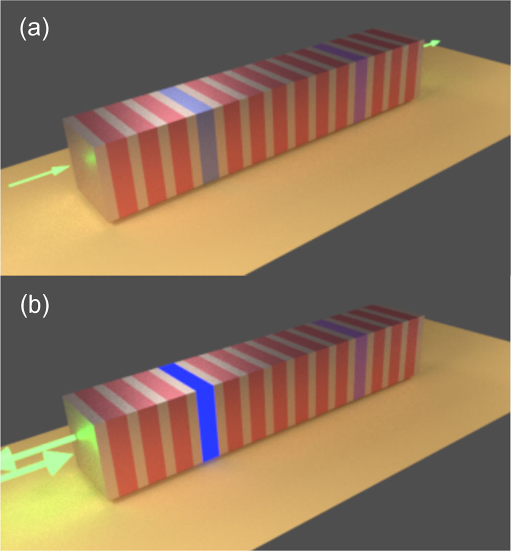
Fig. 1. Multilayer structure involving two coupled cavities with judiciously chosen differential Q factors. (a) At low input intensity (in the linear regime), the photonic circuit supports an EPD and displays resonant transmittance. (b) If the input intensity exceeds the LT, the nonlinearity causes an abrupt lift of the EPD, rendering the photonic circuit highly reflective.

Fig. 2. (a) Schematic of a two-coupled-cavity system (inside a transparent box) connected to two transmission lines. The coupling is asymmetric, i.e., |w1|<|w2|, enforcing differential radiative losses (and therefore Q factors) between the first and the second resonator. The system is designed to support an EPD. (b) Parametric evolution of the frequency difference Δω≡|ω+−ω−| and the corresponding imaginary parts of the two eigenmodes versus the linear detuning Δ [analytical results derived from Eq. (4) are shown by symbols, while the numerical results derived from Eq. (8) are shown by solid lines with a corresponding color]. The solid black line has slope 1/2, while the dashed black line has slope 1 and is drawn in order to guide the eye. Note that Δω≤max{|Im(ω±)|} in the domain where the frequency difference scales as ∝Δ. (c) Transmission spectrum for various detuning strengths Δ (see labels in the inset).

Fig. 3. Parametric evolution of the frequency deference Δω and of the imaginary parts Im(ω±) of the two nonlinear stationary modes of a nonlinear dimer [see Eq. (9)] with α=1, χ=10−4, γ1=0, γ2=γ=1.6×10−3, Ω=0 versus (a) the nonlinear detuning Δ=χ|C1|2 and (b) normalized power N. The solid black line has slope 1/2, while the dashed black line has slope 1 and is drawn in order to guide the eye. Note that Δω≤max{|Im(ω±)|} in the domain where the frequency difference scales as ∝Δ. In the inset of (a), we plot the dependence of χ|C1|2 versus N for each of the two modes ω±. (c) Transmission spectrum of the nonlinear dimer for four representative values of incident power. (d) Transmission T versus incident power |I|2 for four representative frequency detunings. Note that the transmission T associated with the resonant frequency ω=−Ω defines the boundary for all other cases. It drops from unit value at small incident powers to (essentially) zero for high incident powers. In (c) and (d), the parameters of the dimer are the same ones used in Fig. 2(c).

Fig. 4. Transmittance spectra of the system of Fig. 2(a) when the first resonator experiences a nonlinear detuning with nonlinear susceptibility (χ=10−4) and the coupling to the leads is asymmetric. We have used the same parameters as those used in Fig. 3(c). Various incident powers (see inset) are shown. (a) The control parameter is α=γ/2κ=0.4. Note that the transmittance for incident power |I|2=10−2 remains unaffected, while in the corresponding case in Fig. 3(c) we observed a drop by ΔT/T=60%. (b) The control parameter is α=3. In this case the peak transmittance T=34% is already too low for low incident powers. One needs to compare it with the corresponding case in Fig. 3(c) where T=1.

Fig. 5. (a) Resonant split Δf as a function of nD1 refractive index perturbation when loss is higher (red diamonds) or lower (blue triangles) than losses at EPD and when the system is at EPD (purple circles). (b) Transmittance spectra of the free-space multilayer at different incident field intensities. (c) Normalized (with respect to incident field Ei) spatial field intensity distribution within the multilayer at low incident field intensity 104  W/m2 (dark red line) and high incident field intensity 1012  W/m2 (bright red line).

Fig. 6. (a) Transmittance and (b) reflectance of the nonlinear multilayer photonic structure as functions of incident intensity at different frequencies in the vicinity of the resonant frequency of the multilayer f0. The colors indicate the frequency f of the incident wave and are “correlated” with the vertical lines of the same color from Fig. 5(c). The photonic crystal is designed in a way that supports an EPD (i.e., α=1) for low incident powers.

Fig. 7. (a) Re(Δω), Im(ω+) of the nonlinear stationary modes ω± versus the nonlinear detuning Δ=χ|C1|2 for three representative values of α. (b) Same as in (a), but now we report the Im(ω−); (c) same as in (a), but now versus N; and (d) same as in (b), but now versus N.