Spectral singularities have always been an interdisciplinary research theme, offering exciting opportunities to mathematicians, physicists, and engineers [1–3]. While most of the effort has up to now been focused on Hermitian spectral singularities (also known as diabolic points) [4–6], the recent interest in non-Hermitian wave physics has brought to the center of attention a class of spectral singularities known as exceptional point degeneracies (EPDs). Theoretically discussed more than 50 years ago [7], EPDs are non-Hermitian degeneracies emerging when the variation of a control parameter of the system enforces two (or more) eigenvalues and their corresponding eigenvectors to coalesce [7,8]. In fact, the study of EPDs has revealed a variety of fundamental phenomena, which spawned next generation technological developments [9]. Examples range from hypersensitive biosensing [10,11] and navigation devices [12,13] to lasing control [14–16] and unidirectional invisibility [17]. Recently, nonlinear effects in systems containing exceptional points also attracted significant attention [18,19]. In fact, nonlinear systems with non-Hermitian singularities have been investigated for some time, in the framework of critical coupling of optical cavities (see, for example,Ref. [20]).

In this paper, we consider the possibility of using EPD-based photonic circuits with Kerr-effect-like nonlinearities for optical limiting and switching. A typical optical limiter is supposed to transmit low-intensity input light while blocking the light with excessively high intensity, thereby protecting sensitive optoelectronic components or the human eye from laser-induced damage. One common problem with the existing optical limiters is that their limiting threshold (LT) (i.e., incident intensity for which a transmittance drop to small values occurs) [21] is often too high for some important applications. The challenge is to lower the LT while maintaining the ability to withstand high input power without damaging the limiter itself. Here we show that the EPD-based approach allows us to do just that. In addition, the proposed conceptual design can provide an abrupt and fast transition from high transmittance below the LT to nearly total reflectance above the LT. The high reflectance (as opposed to high absorptance) above the LT can prevent overheating and thus drastically increase the limiter damage threshold (LDT).

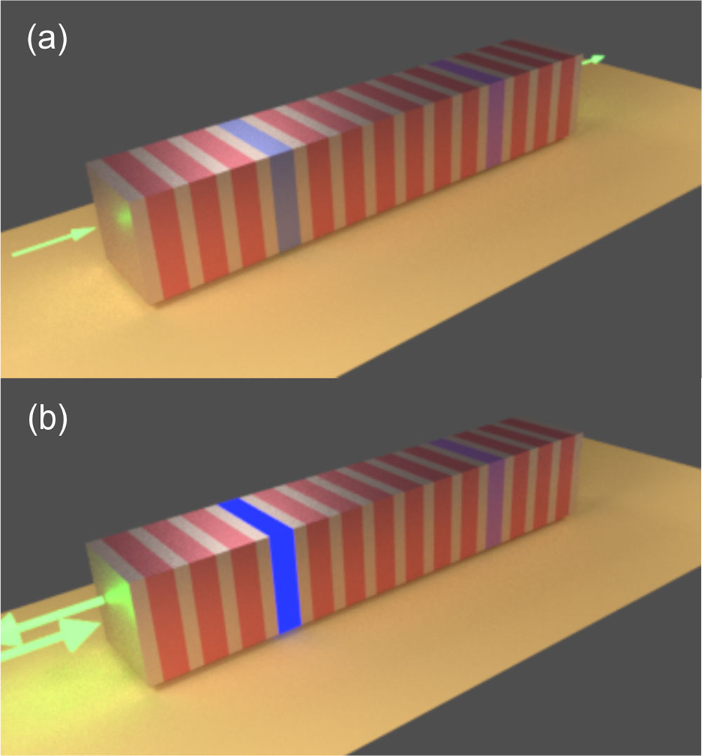
In the proposed design, we implemented a second-order EPD combined with a nonlinear detuning mechanism in a one-dimensional photonic crystal (see Fig. 1). The EPD is achieved by judiciously tailoring differential factors of two defect components of the photonic crystal. One of the defect components is made of a nonlinear (e.g., Kerr-effect-like) material that produces a resonance detuning when the input intensity exceeds the LT. At low input intensity, such that the self-induced nonlinear resonance detuning is proportional to the differential factor, the photonic structure is transparent over a frequency range around the EPD. When, however, the incident intensity exceeds the LT, the two distinct resonant modes emerge when the EPD is lifted due to the nonlinear detuning. One mode undergoes an underdamping-to-overdamping transition due to the differential factor, while the other acquires a narrow resonance width that leads to strong bistability effects, resulting in an abrupt resonance destruction. The EPD-based photonic circuits are therefore excellent candidates for transceiver and other sensitive opto-electronic component protection. Not only do they show an abrupt limiting action, their dynamical range is enhanced due to nearly zero absorption and nearly total reflection of the incident high-power radiation.

In Section 2 we describe the basic idea of the EPD-based approach to optical limiting and demonstrate its efficiency by using a coupled mode theory (CMT) [22]. The analysis first focuses on the linear CMT system. Then, in Section 2.B we proceed with the transport properties of the corresponding nonlinear CMT model. In Section 3 we consider a specific design of a free-space optical limiter based on a one-dimensional multilayer photonic crystal supporting an EPD. Finally, our conclusions are given in Section 4.

We start our analysis by considering two coupled degenerate modes with differential factors. The underlying physical system can be a multilayered photonic crystal with two defect layers (as in Fig. 1) or two coupled optical resonators [as in the transparent box in Fig. 2(a)]). Using a CMT formalism, the system is described by the following effective Hamiltonian : H^=(−Ω−iγ1−κ−κ−Ω−iγ2),(1)where denotes the coupling between the two modes [23,24], is the resonance frequency of each individual cavity (i.e., in the absence of coupling), and is the differential loss between the two cavities. The underlying physical mechanism of the mode losses can be due to ohmic or radiative dissipation (or any other type of loss). We assume, without loss of generality, that .

The supermodes of the composite structure are found via direct diagonalization of Eq. (1). Specifically, we get ω±=−Ω−iγ¯±κ2−(γ2)2,(2)where . The corresponding eigenvectors are v−∝(−iγ−4κ2−γ22κ1);v+∝(−iγ+4κ2−γ22κ1).(3)Equations (2) and (3) imply that at the two modes are degenerate, forming a second-order EPD with and the corresponding degenerate eigenvectors . In the following, we will use the dimensionless ratio as the EPD parameter ( will indicate the formation of an EPD).

Next, we assume that one of the modes experiences a detuning under the condition . To be specific, we assume that the detuning mechanism is associated with the first cavity. The corresponding CMT Hamiltonian is then of the same form as the one of Eq. (1) but with the substitute in the matrix element . Direct diagonalization of allows us to evaluate the influence of the detuning on the supermodes . We have ω±(Δ)=ωEPD−Δ2±−2iγΔ+Δ22,(4)which in the two limiting cases of and takes the following forms: ω+(Δ)≈{ωEPD+(1−i2)γΔ+O(Δ),Δ≪γ−Ω−iγ2,Δ≫γ,(5)and, similarly for , ω−(Δ)≈{ωEPD−(1−i2)γΔ+O(Δ),Δ≪γ−(Ω+Δ)−iγ1,Δ≫γ.(6)Further analysis of Eqs. (5) and (6) reveals that the two supermodes are initially () shifted in opposite directions, away from the EPD frequency with a rate [see the purple stars in Fig. 2(a), showing the frequency split ]. When , the mode keeps moving away from with an increased rate , while comes back at and stays there. In parallel, the linewidth of is initially () decreasing with a rate [see the blue circles in Fig. 2(b)], while the linewidth of increases with the same rate [red triangles in Fig. 2(b)]. Since for , the mode linewidth and the modal spacing scale with in a similar fashion, the two modes can be treated as quasi-degenerate. Under these conditions, the transmittance acquires high values for a frequency range around the EPD. In the opposite limit of , the linewidths of asymptotically approach the values . Therefore, the quality factor of mode () decreases, while that of mode () increases. Consequently, the resonant transmission via mode will degrade, while mode will demonstrate a relatively sharp resonance peak.

The characteristic responses of the eigenmodes to small detunings [see Eqs. (4)–(6)] also manifest themselves in the case of scattering setup, i.e., when each resonator is coupled to a transmission line; see Fig. 2(a). In this setting, the eigenmodes turn to resonant modes, whose resonant frequencies and linewidths are associated with the real and imaginary parts of the poles of the scattering matrix . The latter is expressed in terms of the Hamiltonian of the isolated system [25] as S^=−I^2−iW^T1H^eff−ωI^2W;H^eff=H^(Δ)+Λ−i2W^W^T,(7)where is the identity matrix and describes the resonator-lead coupling. Its elements are , where are dimensionless coupling strengths and . Finally, the renormalization matrix originates from the coupling of the system to the leads, and it is specific to the properties of the transmission line. For example, when the transmission lines consist of coupled resonator optical waveguide (CROW) arrays [see Fig. 2(a)], supporting propagating waves with a dispersion relation ( is the wavevector and is the coupling constant between the resonators in the leads), the group velocity is , while .

Equation (7) allows us to identify the poles of the scattering matrix as the zeros of the secular equation: det[H^eff−ωI2]=0,(8)which, in the case of CROW transmission lines, needs to be evaluated numerically. In fact, the analysis can be further simplified if we consider a wide band approximation corresponding to . In this case, the tight-binding dispersion reduces to the free-space dispersion, and the analysis of the poles of boils down to the study of the eigenvalues of . Since is diagonal with coupling elements , the eigenvalues of are essentially the same as the eigenvalues of with the substitutions and . Therefore, the resonant modes are affected by the detuning in the same manner as the eigenfrequencies of .

We have calculated the resonances of the scattering setup of Fig. 2(a) by numerically solving Eq. (8) for CROW transmission lines. Furthermore, we assumed that the underlying physical origin of the differential factor of the two modes is due to their asymmetric coupling with the transmission lines and , while [in Eq. (1)] and . In our simulations we assumed that the resonant frequency of the two resonators is . Our results for the frequency splitting versus are shown with symbols in Fig. 2(b). In the same figure, we also report the parametric evolution of of the eigenmodes of [see Eq. (1)] with equivalent mode losses . The nice overlap validates the prediction that the parametric behavior with , of the resonant modes and the eigenmodes of , is the same.

The effect of on the resonance splitting has direct consequences to the shape of the transmittance spectrum ; see Fig. 2(c). Specifically, for , shows only one resonance peak associated with the EPD. The position of this peak is at , and its linewidth is . As increases, the EPD is lifted. However, the emerging two resonant peaks at are not resolved as long as . This is because the resonant mode linewidths are larger than the mode spacing ; see Fig. 2(b). For larger values of , the resonance peaks are shifted apart from each other, and their linewidths acquire fixed values where . In this regime, the transmittance peak associated with the resonant mode broadens to the linewidth and becomes suppressed due to the decrease of the factor of the mode. On the other hand, the resonance peak associated with narrows to the linewidth . Either way, both modes acquire reduced transmittance due to the strong resonance detuning between the modes. Alternatively, the reduced transmittance for large values can be seen as a consequence of an increasing impedance mismatch between the two resonators, which leads to an enhanced reflection.

In the previous analysis we did not discuss the physical origin of the mode detuning in one of the cavities/modes. For example, it can be induced externally by a temperature or a pressure variation, by an injected current that changes the permittivity of the resonator, or as a consequence of an externally applied electric field. In this subsection, we will focus on the case where the detuning is self-induced via a nonlinear light–matter interaction. Specifically, we will assume that the detuning is associated with a nonlinear mechanism, like the Kerr effect, i.e., , where is the field intensity at the cavity.

First, we will analyze the stationary nonlinear supermodes of the two coupled resonators. For simplicity we will assume that and . We request the total power normalization such that . The stationary nonlinear eigenmodes of this system can be evaluated using the following CMT equations: [−Ω−χ|C1|2−κ−κ−Ω−iγ][C1C2]=ω[C1C2],(9)where, without loss of generality, we will assume that is real and . Straightforward manipulations of Eq. (9), together with the normalization condition, lead to the following transcendental equation: (η+ηy)2+α2=11−y2;tan(ϕ)=αyη(1+y),(10)where have been parametrized in terms of the variable as , while their relative phase is given by the second equation in Eq. (10). Above, we have defined and . We note that for , the EPD is formed when .

We request the solutions of the first Eq. (10) to be real. Their direct substitution in one of the equations in Eq. (9) allows us to calculate the nonlinear stationary eigenfrequencies of the system described by Eq. (9). The latter are given as ω±/κ=−Ω/κ−η(1+y±)2/y±−iα(1−y±).(11)In Fig. 3(a), we show (for ) the behavior of (stars) and (triangles and circles) resulting from Eq. (11) versus the nonlinear detuning . In this calculation, the value of , and therefore of the detuning, determine the total power . The latter might have two different values for a fixed (see inset) due to the presence of bistabilities—a phenomenon typical to nonlinear optics. In the same figure, we also plot (solid lines of blue and red colors for imaginary parts and violet for the real part) the predictions from the linear analysis [see Eq. (4)] assuming a specific value. We also report in Fig. 3(b) the same quantities versus by identifying the values [see inset in Fig. 3(a)] that are associated with a fixed . In both cases, the resonance shift is initially smaller than the resonance linewidths, indicating that the two modes are indistinguishable from one another. We find that the behavior of versus the detuning is essentially the same as the one found for the corresponding linear system. In fact, the similarities with the linear problem extend also to the regime where . We find that is stabilized at and acquires a broad linewidth , which indicates a decrease of the factor and therefore suppression of the transmittance [see Fig. 3(c) and related discussion/analysis below]. On the other hand, moves away from , while its linewidth narrows to . In the following, we will show that the enhancement of the factor of has dramatically different consequences on the transmittance spectrum as compared to the linear case (see below).

Next, we analyze the transport properties of the CMT system described by Eq. (9). We consider the same scattering setup with semi-infinite CROW transmission lines as shown in Fig. 2(a). We assume that the differential factor is due to an asymmetric coupling to the leads while . We also assume the same parameter values as those in the case of the linear scattering setup analyzed in Fig. 2(c).

For the calculation of the transmittance , we employ the so-called backward transfer map [26,27], where we have assumed that the incident wave is entering the dimer structure from the left transmission line. We also assume that the outgoing field at the right transmission line takes the form (), where is the transmission amplitude and indicates the field amplitude at the th resonator. A backward iteration of the CMT equations describing the setup allows us to evaluate the wave at the left transmission line, (), where I and r are the incident and reflected amplitudes, respectively. Thus, represents the incoming intensity, and is the reflectance. Straightforward algebra leads to the following expression for the transmittance : T=|2sin(k)F·G(T)κtl−κtlw1w2|2,k>0,(12)where , , and . Equation (12) is a transcendental equation with respect to and has to be solved numerically. Since no dissipative losses are involved, the reflectance can be evaluated as . Typically, these nonlinear variations of the real part of the refraction index are accompanied by variations in the imaginary part of the index due to Kramers–Kronig (KK) relation. In our analysis, these variations of the imaginary refractive index are disregarded in order to highlight the proposed limiting mechanism. We have checked, however, that the addition of these nonlinear losses does not have any qualitative impact on the performance of the device. In case of high incident intensities, the growth of the absorption due to the KK nonlinear losses will transition the system to the overdamped regime. As a consequence, the system is still rendered strongly reflective and not absorptive.

In Fig. 3(c), we report some representative transmittance spectra for the nonlinear dimer at and . All other parameters are the same as the ones used in Fig. 2(c). For low incident powers, the transmittance shows the same behavior as in the linear case (), i.e., a single quasi-degenerate peak at , where . As the incident power increases, the two resonance peaks at separate from each other: the frequency position of remains unaffected from the incident power and the self-induced nonlinear detuning, while its linewidth increases until it reaches its asymptotic value . This decline in the factor of the resonant mode leads eventually to a gradual suppression of the transmittance peak. The other emerging resonant mode, associated with , is “pushed away” from and becomes “sharper” due to the narrowing of its linewidth. In the nonlinear scenario, however, this “upgrade” to a high triggers a nonlinear bistability, which leads to an abrupt suppression of the resonance peak. As a result, the structure demonstrates a (near-) unity reflectance at for high-power incident radiation (large nonlinear detuning). An overview of the transmittance versus the incident power for various frequencies is shown in Fig. 3(d). The results indicate that the optimal limiting behavior (high transmittivity for low powers and transmittivity drop for high incident powers) occurs for a range of frequencies around the EPD at .

We stress that the transition from a (near-) unity transmittance to a (near-) unity reflectance is associated with the presence of the EPD. In order to clarify this point, we present an analysis of the transport properties of the two nonlinear coupled resonant modes for and ; see Figs. 4(a) and 4(b). A further insight is gained by an extended analysis of the parametric evolution of the nonlinear stationary modes of Eq. (9) versus the nonlinear detuning (and also the total mode power ). This analysis is reported in Appendix A (see also Fig. 7). For [Fig. 4(a)], both modes have the same linewidth (under-damped regime) up to a nonlinear detuning . As a result the transmission spectrum is unaffected in this range. It is instructive to compare the transmittance data shown by the blue and purple filled circles in Fig. 4(a) with the transmittance spectra at the same incident powers for [see the same color symbols in Figs. 3(c)]. In the latter case, the increase in the incident power leads to a transmittance drop by . When increases further (), the bifurcate to their asymptotic values. Similarly to the case, one of the modes acquires a narrow linewidth and gets destroyed due to nonlinear effects while the other one is “spoiled” due to an increase of its linewidth. This linewidth increase, though, is less steep as compared to the case, and therefore the suppression of the corresponding resonance peak is gradual. When [see Fig. 4(b)], the mode is extremely sharp, even for small incident powers (nonlinear detuning ), and therefore it becomes bistable and is immediately destroyed due to the presence of nonlinearities [see the purple line drops on the left of Fig. 4(b)]. At the same time, has the maximum linewidth due to the strong coupling to the leads, and its resonance peak is well below unity (). We conclude that the presence of an EPD (i.e., ) combined with the nonlinear bistabilities can be used in order to design a power limiter with optimal transport characteristics: (almost) perfect transmittance at low incident powers and (almost) perfect reflectance at high incident powers. We point out that the coexistence of nonlinearity with losses (or asymmetric coupling) can produce an asymmetric transmission leading to another functionality of the proposed photonic circuit [28].

The theoretical understanding of the interplay between the nonlinearities and the existence of EPDs in the transport properties of two coupled resonant modes allows us to propose a design for a free-space photonic limiter as opposed to waveguided or localized-CROW-based designs. The structure consists of a multilayer one-dimensional photonic crystal with two optically identical defect cavities placed symmetrically with respect to a mirror plane; see Fig. 1. The geometric arrangement of the photonic crystal is , where and denote quarter-wave thick layers. The two cavities are designed in a way that they support defect modes in the middle of the band-gap of the photonic crystal. Under such conditions, the two degenerate defect modes are isolated from the rest of the Fabry–Perot modes, and thus they can be described by the two-level system of Eqs. (1) and (9). Finally, the coupling strength that controls their mutual interaction is dictated by the number of layers between the two cavities. Specifically, we have that , where is the number of in-between layers and is the so-called localization length of these defect modes.

The designed Fabry–Perot cavities are both tuned at resonant frequency (), and the and layers denote quarter-wave-thick layers of with refractive index [29] and with refractive index [30]. The first cavity has a nonlinear half-wave-thick ZnS defect layer with intensity-dependent refractive index [31]. is the electric field intensity at position inside the layer, which is responsible for the nonlinear detuning . The second Fabry–Perot cavity has tiny (radiative or ohmic) losses modeled in our simulations via a complex refractive index of the half-wave-thick doped defect layer. The coupling coefficient between two Fabry–Perot cavities is controlled via the number of bilayers () between the two defect layers and .

First, we identify the number , of bilayers and loss strength , which leads to the formation of an EPD in the low incident power limit. In this case, the system is linear, i.e., is essentially constant and independent of the incident power. The EPD condition has been identified via a detail scaling analysis of the resonance splitting versus for various values of . The detuning has been controlled by “manually” changing the value of , i.e., . The photonic design that supports an EPD has been identified as the configuration where for , while for . In our case, this behavior is achieved when and for , number of bilayers. In Fig. 5(a) we show the results of this analysis for three different cases corresponding to , 1, and 1.2. In the former case, the resonant modes are not degenerate for , and they acquire a fixed resonant split that remains unaffected from any index modulation up to . Above this value, the frequency difference between the two resonant modes increases linearly with ; see Fig. 5(a). In contrast, for , the resonant modes are degenerate for , and their degeneracy is lifted very slowly, following a linear relation with detuning , i.e., .

Next we consider the nonlinear transport properties of the multilayer system once it is brought at the EPD (). We assume that the defect has a nonlinear index of refraction corresponding to ZnS material (see above). In our simulations, we have involved a backward transfer matrix approach [26,27] for the evaluation of transmittance and reflectance . Figure 5(b) shows the transmission spectra for three representative incident powers. The results confirm the predictions of the two-mode CMT modeling [see Fig. 3(c)]. Namely, for low incident powers, the transmittance is (almost) unity at the EPD frequency ; for higher incident powers the resonant peak splits in two, with the first one remaining at while the other one is shifted away. The first peak broadens, leading to a deterioration of the resonant mode and a consequent suppression of the transmittance. The second transmission peak is abruptly suppressed, showing a bistable behavior due to the presence of the nonlinearity. The destruction of the resonant defect modes is also evident from the spatial intensity distribution illustrated in Fig. 5(c). In this figure we show the low-intensity incident scattering profile (dark red line) at resonant mode together with the scattering field corresponding to high incident powers (bright red line). In the former case, the intensity is exponentially enhanced at the vicinity of the defect layers and , leading to a strong enhancement of the nonlinearity and therefore to strong nonlinear detuning. Further increase of the latter due to higher incident radiation powers is the source of the resonance destruction (bright red line) and consequent transmission resonant peak suppression. As a result, the structure turns to an (almost) completely reflective one at high incident powers.

An overview of the transmittance () and reflectance () in the vicinity of the resonant frequency as functions of input intensity is shown in Figs. 6(a) and 6(b). At the resonant frequency [yellow lines in panels Figs. 6(a) and 6(b)], the transmittance decay at high intensities is correlated with an abrupt growth of the reflectance. At lower frequencies [blue and orange lines in panels Figs. 6(a) and 6(b)], the transmittance demonstrates bistable behavior at high incident intensities, and its magnitude is highly suppressed over a broad intensity range, implying that in this region the multilayer provides high reflectivity at any incident intensity level. At frequencies above , the system does not show any bistable behavior [purple line in panels Figs. 6(a) and 6(b)], and the transmittance is highly suppressed across a broad incident irradiance range.

We can therefore conclude that the proposed photonic structure can be utilized as a power limiter with an extremely sharp transition from a high (near-unity) resonant transmittance to a broadband reflectance. As opposed to other reflective photonic limiters, this proposal does not involve absorption growth at any incident intensity levels, and it therefore has an enhanced dynamical range.

In this paper, we have analyzed an EPD-based photonic circuit and demonstrated its efficiency for optical limiting and switching. The circuit consisted of two optically identical cavities with differential factors embedded in a multilayer structure. One of the cavities involves a nonlinear component that is responsible for triggering a resonant detuning once the incident radiation intensity is above a critical value. For low input intensities (linear regime), the structure displays strong EPD-related resonant transmittance. For high input intensities, the light-induced detuning lifts the EPD. Specifically, one of the emerging resonances is abruptly suppressed due to nonlinear instabilities, while the other becomes overdamped. This renders the photonic circuit highly reflective for a broad frequency range, with negligible absorption, preventing the circuit from overheating at high input light intensities. The limiting threshold, which defines the transition from resonant transparency to broadband near-complete reflectivity, can be tailored by arranging the thicknesses of the two defect cavities. Specifically, an increase in nonlinear layer thickness results in enhanced detuning of nonlinear resonant frequency and sharper transition to the reflective state. The advantages of the proposed design include the possibility of a much lower limiting threshold (LT) and much higher limiter damage threshold (LDT), compared to those achievable with passive limiters or switches using optical materials with nonlinear absorption. Finally, based on a nonlinear coupled mode theory, we have developed analytical designing tools for the photonic structures with EPD.

Acknowledgment. The authors acknowledge useful discussions with S. Ali, who participated at the initial stage of the project. We also acknowledge useful discussions with Dr. R. Sher on material properties.

References

[1] A. Mostafazadeh. Physics of spectral singularities. Geometric Methods in Physics, 145-165(2015).
[23] The most general non-Hermitian coupled mode theory could involve complex coupling coefficients [24]. In our heterostructure (involving two defect layers), however, the modeling of Eq. (1) is sufficient for capturing all transport features (see Section 3).