Cubic–quartic optical soliton perturbation and modulation instability analysis in polarization-controlled fibers for Fokas–Lenells equation

Khalil S. Al-Ghafri; Edamana V. Krishnan; Anjan Biswas

doi:10.1051/jeos/2022008

Abstract

The objective of this study is to investigate miscellaneous wave structures for perturbed Fokas–Lenells equation (FLE) with cubic-quartic dispersion in polarization-preserving fibers. Based on the improved projective Riccati equations method, various types of soliton solutions such as bright soliton, combo dark–bright soliton, singular soliton and combo singular soliton are constructed. Additionally, a set of periodic singular waves are also retrieved. The dynamical behaviors of some obtained solutions are depicted to provide a key to understanding the physics of the model. The modulation instability of the FLE is reported by employing the linear stability analysis which shows that all solutions are stable.The objective of this study is to investigate miscellaneous wave structures for perturbed Fokas–Lenells equation (FLE) with cubic-quartic dispersion in polarization-preserving fibers. Based on the improved projective Riccati equations method, various types of soliton solutions such as bright soliton, combo dark–bright soliton, singular soliton and combo singular soliton are constructed. Additionally, a set of periodic singular waves are also retrieved. The dynamical behaviors of some obtained solutions are depicted to provide a key to understanding the physics of the model. The modulation instability of the FLE is reported by employing the linear stability analysis which shows that all solutions are stable.

1　Introduction

Recently, nonlinear optics has become one of the important fields of science that have wide range of physical and engineering applications. The significance of this field has been enhanced since the appearance of optical fiber as a common type of optical waveguide that transmits light and signals over longe distances [1, 2]. Further to this, the continuous theoretical and experimental research works confirm that optical fiber has potential influences on developing photonic and optoelectronic devices [3–6]. One of the diagnostic tools to examine the physical properties of optical fiber is the optical pulses. The controllable interaction of dispersion and nonlinearity of the pulse propagation leads to the formation of stable and undistorted pulses known as soliton. There are several mathematical models that study the dynamic of soliton in optical fibers. One of these models that is accounted as a generalized form of the nonlinear Schrödinger equation is the Fokas–Lenells equation (FLE). In literature, FLE is dealt with by many authors to obtain exact solutions by utilizing various powerful techniques. The employed integration schemes in the previous studies are Sine-Gordon expansion method, Riccati equation method, mapping method, trial equation method, Kudryashov’s method, semi-inverse variational principle, modified simple equation method, Laplace-Adomian decomposition method, auxiliary equation method and many others. For more details, readers are referred to references [7–18].

Soliton propagation along an optical fiber can be subject to the low count of chromatic dispersion (CD) which severely affects the transmission process. To overcome this effect, a variety of novel techniques have recently been proposed. One of the most popular technologies employed in the research studies is based on adding another form of dispersion such as Bragg gratings dispersion, pure–cubic dispersion, pure–quartic dispersion, cubic–quartic dispersion and many others. For example, the combination of fourth-order dispersion (4OD) and third-order dispersion (3OD) terms can completely compensate for low CD and gives rise to creation of the so-called cubic–quartic (CQ) solitons, see the references [19–24]. Later, the model of FLE is developed to include 4OD and 3OD terms and that means CQ solitons can be constructed in polarization preserving fibers [25–27]. The current study mainly discusses CQ-FLE with perturbation terms of Hamiltonian type. The proposed model takes the form(1) $i Ψ_{t} + ia Ψ_{xxx} + b Ψ_{xxxx} + | Ψ |^{2} (c Ψ + id Ψ_{x}) = i {α Ψ_{x} + λ (| Ψ |^{2 n} Ψ)_{x} + μ (| Ψ |^{2 n})_{x} Ψ},$ where Ψ(x, t) is is a complex-valued function representing optical soliton profile. The independent variables x and t denote the distance along the fiber and the elapsed time, respectively. The first term indicates the time evolution while the terms with a and b account for the third- and fourth-order dispersions. The nonlinear influence has the form of Kerr law and is given by the coefficient of c. The term with d is the coefficient of nonlinear dispersion. On the right-hand side of equation (1), the perturbation terms with α, λ and μ are defined as inter-modal dispersion, self-steepening effect and higher-order dispersion, respectively. The parameter n represents the full nonlinearity effect and $i = \sqrt{- 1}$ .

The model (1) is investigated with the help of the improved projective Riccati equations method [28, 29] to derive distinct exact solutions. The rest of this paper is organized as follows. In Section 2, we describe the suggested scheme. Section 3 demonstrates how the FLE is reduced to a simple form using the traveling wave transformation. In Section 4, various solution expressions illustrating different wave structures are extracted. In Section 5, the modulation instability by means of standard linear stability analysis is examined. Section 6 displays the remarks and discussion of the obtained results. Finally, our conclusion is given in Section 7.

2　Elucidation of scheme

Herein, we present the process of applying the improved projective Riccati equations method as follows. Consider a nonlinear evolution equation (NLEE) in the form(2) $P (u, u_{t}, u_{x}, u_{xx}, u_{xt}, u_{tt}, u_{xxx} \dots) = 0,$ where u = u(x, t) is an unknown function and P is a polynomial in u and its various partial derivatives.

Based on the traveling wave transformation given by(3) $u (x, t) = U (ξ), ξ = x - ct,$ the NLEE (2) reduces to a nonlinear ordinary differential equation (NLODE) of the form(4) $Q (U, U', U'', U''', \dots) = 0,$ where prime denotes the derivative with respect to ξ.

We assume that equation (4) has a solution in the form of a finite series as(5) $U (ξ) = a_{0} + b_{0} f (ξ) g (ξ) + \sum_{j = 1}^{m} [a_{j} f^{j} (ξ) + b_{j} g^{j} (ξ)],$ where a_j, b_j, (j = 0, 1, 2, …, m) are constants to be determined. The parameter m is a positive integer which can be identified by balancing the highest order derivative term with the nonlinear term in equation (4).

The variables f(ξ) and g(ξ) satisfy the the following improved projective Riccati equations(6) $\begin{matrix} f' (ξ) = δ A g^{2} (ξ), g' (ξ) = - Af (ξ) g (ξ) - \frac{B}{A} g (ξ) (R - Bf (ξ)), \\ g^{2} (ξ) = δ [\frac{1}{A^{2}} (R - Bf (ξ))^{2} - f^{2} (ξ)], \end{matrix}$ $$ \begin{array}{c}f\mathrm{\prime}(\xi )={\delta A}{g}^2(\xi ),\hspace{1em}\enspace g\mathrm{\prime}(\xi )=-{Af}(\xi )\enspace g(\xi )-\frac{B}{A}\enspace g(\xi )\enspace (R-{Bf}(\xi )),\hspace{1em}\\ {g}^2(\xi )=\delta \left[\frac{1}{{A}^2}\enspace (R-{Bf}(\xi ){)}^2-{f}^2(\xi )\right],\end{array} $$ where A, B and R are arbitrary constants and δ = ±1. The third equation in the system (6), which gives the relation between the functions f(ξ) and g(ξ), represents the first integral of the couple ODEs in this system.

The set of equations (6) is found to possess solutions in the form(7) $f_{1} (ξ) = \frac{R \tanh (Rξ)}{A + B \tanh (Rξ)}, g_{1} (ξ) = \frac{R sech (Rξ)}{A + B \tanh (Rξ)},$ which implies δ = 1, and(8) $f_{2} (ξ) = \frac{R \coth (Rξ)}{A + B \coth (Rξ)}, g_{2} (ξ) = \frac{R csch (Rξ)}{A + B \coth (Rξ)},$ provided that δ = −1.

Substituting (5) along with (6) into equation (4) gives a polynomial in f^j (ξ) and f^j (ξ) g(ξ). Then, we equate each coefficient of f^j (ξ) and f^j (ξ)g(ξ) in this polynomial to zero to get a set of algebraic equations for a_j, b_j. Finally, solving this system of equations, we obtain various exact solutions of equation (2) according to (7) and (8).

3　Traveling wave reduction of the model

Now, we aim to reduce the complex form of the model (1) to an NLODE with a view to deriving the optical soliton solutions. Therefore, we assume the traveling wave transformation of the form(9) $Ψ (x, t) = ψ (ξ) e^{iϕ (x, t)},$ where ψ(ξ) accounts for the amplitude of the soliton while ϕ(x, y, t) denotes the phase component. The wave variable ξ is given by(10) $ξ = x - ν t,$ and the function ϕ(x, y, t) is introduced as(11) $ϕ (x, y, t) = - κ x + ω t + θ,$ where the parameters ν, κ, ω and θ represent the soliton velocity, frequency, wave number and phase constant, respectively.

Substituting (8) into equation (1) leads to a couple of equations for real and imaginary parts given, respectively, as(12) $b ψ^{iv} + (3 aκ - 6 b κ^{2}) ψ'' - (ω + α κ + a κ^{3} - b κ^{4}) ψ + (c + dκ) ψ^{3} - λ κ ψ^{2 n + 1} = 0,$ (13) $(a - 4 aκ) ψ''' - (α + ν + 3 a κ^{2} - 4 b κ^{3}) ψ' + d ψ^{2} ψ' - (2 nμ + (2 n + 1) λ) ψ^{2 n} ψ' = 0,$ where the prime denotes the derivative with respect to ξ. The system of equations (12) and (13) is reduced to(14) $b ψ^{iv} + 6 b κ^{2} ψ'' - (ω + α κ + 3 b κ^{4}) ψ + (c + dκ - λ κ) ψ^{3} = 0,$ with the expression for the velocity of the soliton presented as(15) $ν = - α - 8 b κ^{3},$ under the constraints(16) $n = 1,$ (17) $a = 4 bκ,$ (18) $d - 2 μ - 3 λ = 0 .$

4　Solutions of the model

Now, we embark on deriving the solutions of the perturped CQ-FLE through implementing the improved projective Riccati equations method stated in Section 2. The proposed technique is basically used to handle equation (14) and then its obtained solutions are plugged into the transformation (9) so as to extract the optical solitons of the governing model.

According to the series formula given in (5) and the balance between the terms ψ^iv and ψ³ in equation (14), this leads to m = 2. Hence, the general solution form of equation (14) reads(19) $ψ (ξ) = a_{0} + b_{0} f (ξ) g (ξ) + \sum_{j = 1}^{2} [a_{j} f^{j} (ξ) + b_{j} g^{j} (ξ)] .$

Substituting (19) together with equations (6) into equation (14) gives rise to an equation having different powers of f^lg^s. Collecting all the terms with the same power of f^lg^s together and equating each coefficient to zero, yields a set of algebraic equations. Solving these equations simultaneously leads to the following results.

Set I. If δ = 1, then the following cases of solutions in the hyperbolic secant and tangent functions are retrieved.

Case 1.

(20) $a_{0} = a_{1} = a_{2} = b_{2} = 0, b_{0} = \pm 2 \sqrt{\frac{30 b (A^{2} - B^{2})^{3}}{A^{2} (c + dκ - λ κ)}}, b_{1} = \frac{b_{0} RB}{A^{2} - B^{2}}, ω = - α κ + \frac{24}{25} b κ^{4}, R = \pm \sqrt{\frac{3}{5}} κ .$

Inserting (20) in accompany with (7) into (19) yields(21) $Ψ (x, t) = \pm 2 R^{2} \sqrt{\frac{30 b (A^{2} - B^{2})}{c + dκ - λ κ}} \frac{A \tanh (Rξ) sech (Rξ) + B sech (Rξ)}{{(A + B \tanh (Rξ))}^{2}} e^{iϕ (x, t)},$ where b(A² − B²)(c + dκ − λκ) > 0, ξ = x + (α + 8bκ³)t and $ϕ (x, t) = - κ x - (α κ - \frac{24}{25} b κ^{4}) t + θ$ .

Case 2.

(22) $b_{0} = b_{1} = b_{2} = 0, a_{0} = \frac{3 a_{2} κ^{2}}{10 (A^{2} - B^{2})}, a_{1} = \frac{2 a_{2} RB}{A^{2} - B^{2}}, a_{2} = \pm \frac{2 (A^{2} - B^{2})^{2}}{A^{2}} \sqrt{- \frac{30 b}{c + dκ - λ κ}}, ω = - α κ - \frac{219}{25} b κ^{4}, R = \pm \sqrt{- \frac{3}{10}} κ .$

Plugging (22) along with (7) into (19) brings about(23) $Ψ (x, t) = \pm 2 (A^{2} - B^{2}) R^{2} \sqrt{- \frac{30 b}{c + dκ - λ κ}} \times \frac{\sec h^{2} (Rξ)}{{(A + B \tanh (Rξ))}^{2}} e^{iϕ (x, t)},$ where b(c + dκ − λκ) < 0, ξ = x + (α + 8bκ³)t and $ϕ (x, t) = - κ x - (α κ + \frac{219}{25} b κ^{4}) t + θ$ .

Case 3.(24) $a_{1} = a_{2} = b_{0} = b_{1} = 0, a_{0} = - \frac{b_{2} (10 R^{2} + 3 κ^{2})}{30 (A^{2} - B^{2})}, b_{2} = \pm 2 (A^{2} - B^{2}) \sqrt{- \frac{30 b}{c + dκ - λ κ}}, ω = - α κ - 18 b R^{2} κ^{2} - \frac{6}{5} b κ^{4}, 40 R^{4} - 30 R^{2} κ^{2} + 9 κ^{4} = 0 .$

Substituting (24) together with (7) into (19) generates(25) $Ψ (x, t) = \pm \sqrt{- \frac{30 b}{c + dκ - λ κ}} \times \{\frac{10 R^{2} + 3 κ^{2}}{15} - \frac{2 (A^{2} - B^{2}) R^{2} \sec h^{2} (Rξ)}{{(A + B \tanh (Rξ))}^{2}}\} e^{iϕ (x, t)},$ where b(c + dκ − λκ) < 0, ξ = x + (α + 8bκ³)t and $ϕ (x, t) = - κ x - (α κ + 18 b R^{2} κ^{2} + \frac{6}{5} b κ^{4}) t + θ$ .

Case 4.(26) $b_{0} = b_{1} = b_{2} = 0, a_{0} = \frac{3 a_{2} κ^{2}}{10 (A^{2} - B^{2})}, a_{1} = \frac{2 a_{2} RB}{A^{2} - B^{2}}, a_{2} = \pm \frac{2 (A^{2} - B^{2})^{2}}{A^{2}} \sqrt{- \frac{30 b}{c + dκ - λ κ}}, ω = - α κ - \frac{219}{25} b κ^{4}, R = \pm \sqrt{- \frac{3}{10}} κ .$

Putting (26) in addition to (7) into (19) gives us the soliton solution (23).

Case 5.(27) $a_{0} = a_{1} = a_{2} = 0, b_{0} = \pm \frac{b_{2} \sqrt{B^{2} - A^{2}}}{A}, b_{1} = \pm \frac{b_{2} RB \sqrt{B^{2} - A^{2}}}{A (A^{2} - B^{2})}, b_{2} = \pm (A^{2} - B^{2}) \sqrt{- \frac{30 b}{c + dκ - λ κ}}, ω = - α κ - \frac{219}{25} b κ^{4}, R = \pm \sqrt{- \frac{6}{5}} κ .$

Plugging (27) and (7) into (19) leads to(28) $Ψ (x, t) = \pm R^{2} \sqrt{\frac{30 b (A^{2} - B^{2})}{c + dκ - λ κ}} \times \frac{sech (Rξ) [B + A \tanh (Rξ) \pm \sqrt{B^{2} - A^{2}} sech (Rξ)]}{{(A + B \tanh (Rξ))}^{2}} e^{iϕ (x, t)},$ where b(c + dκ − λκ) < 0, A² < B², ξ = x + (α + 8bκ³)t and $ϕ (x, t) = - κ x - (α κ - \frac{219}{25} b κ^{4}) t + θ$ .

Case 6.(29) $b_{2} = 0, a_{0} = \frac{6 b_{0} κ^{2}}{5 A \sqrt{B^{2} - A^{2}}}, a_{1} = \pm \frac{2 b_{0} RB \sqrt{B^{2} - A^{2}}}{A (A^{2} - B^{2})}, a_{2} = \pm \frac{b_{0} \sqrt{B^{2} - A^{2}}}{A}, b_{1} = \frac{b_{0} RB}{A^{2} - B^{2}}, b_{0} = \pm \sqrt{\frac{30 b (A^{2} - B^{2})^{3}}{A^{2} (c + dκ - λ κ)}}, ω = - α κ - \frac{219}{25} b κ^{4}, R = \pm \sqrt{- \frac{6}{5}} κ .$

Substituting (29) in accompany with (7) into (19) produces the soliton solution (28).

Case 7.(30) $b_{0} = b_{1} = b_{2} = 0, a_{0} = - \frac{a_{2} (20 R^{2} A^{2} - 30 R^{2} B^{2} - 3 A^{2} κ^{2})}{30 (A^{2} - B^{2})^{2}}, a_{1} = \frac{2 a_{2} RB}{A^{2} - B^{2}}, a_{2} = \pm \frac{2 (A^{2} - B^{2})^{2}}{A^{2}} \sqrt{- \frac{30 b}{c + dκ - λ κ}}, ω = - α κ - 18 b R^{2} κ^{2} - \frac{6}{5} b κ^{4}, 40 R^{4} - 30 R^{2} κ^{2} + 9 κ^{4} = 0 .$

Inserting (30) along with (7) into (19), we secure(31) $\begin{matrix} Ψ (x, t) = & \pm \sqrt{- \frac{30 b}{c + dκ - λ κ}} \{\frac{20 A^{2} R^{2} - 3 A^{2} κ^{2} - 30 B^{2} R^{2}}{15 A^{2}} \\ - \frac{2 (A^{2} - B^{2}) R^{2} \tanh (Rξ) \{(A^{2} + B^{2}) \tanh (Rξ) + 2 AB\}}{A^{2} {(A + B \tanh (Rξ))}^{2}}\} e^{iϕ (x, t)}, \end{matrix}$ where b(c + dκ − λκ) < 0, ξ = x + (α + 8bκ³)t and $ϕ (x, t) = - κ x - (α κ + 18 b R^{2} κ^{2} + \frac{6}{5} b κ^{4}) t + θ$ .

Case 8.(32) $\begin{matrix} a_{1} = a_{2} = 0, a_{0} = - \frac{b_{2} (5 R^{2} + 6 κ^{2})}{30 (A^{2} - B^{2})}, b_{0} = \pm \frac{b_{2} \sqrt{B^{2} - A^{2}}}{A}, b_{1} = \pm \frac{b_{2} RB \sqrt{B^{2} - A^{2}}}{A (A^{2} - B^{2})}, \\ b_{2} = \pm (A^{2} - B^{2}) \sqrt{- \frac{30 b}{c + dκ - λ κ}}, ω = - α κ - \frac{9}{2} b R^{2} κ^{2} - \frac{6}{5} b κ^{4}, 5 R^{4} - 15 R^{2} κ^{2} + 18 κ^{4} = 0 . \end{matrix}$

Substituting (32) as well as (7) into (19) provides the soliton solution(33) $\begin{matrix} Ψ (x, t) = \pm \sqrt{- \frac{30 b}{c + dκ - λ κ}} \{\frac{5 R^{2} + 6 κ^{2}}{30} \pm \frac{R^{2} \sqrt{B^{2} - A^{2}} sech (Rξ) [B + A \tanh (Rξ)]}{{(A + B \tanh (Rξ))}^{2}} \\ - \frac{R^{2} (A^{2} - B^{2}) \sec h^{2} (Rξ)}{{(A + B \tanh (Rξ))}^{2}}\} e^{iϕ (x, t)}, \end{matrix}$ where $b (c + dκ - λ κ) < 0, A^{2} < B^{2}, ξ = x + (α + 8 b κ^{3}) t$ and $ϕ (x, t) = - κ x - (α κ + \frac{9}{2} b R^{2} κ^{2} + \frac{6}{5} b κ^{4}) t + θ$ .

Case 9.

(34) $\begin{matrix} b_{2} = 0, a_{0} = \frac{b_{0} (25 R^{2} A^{2} - 30 R^{2} B^{2} - 6 A^{2} κ^{2})}{30 A (A^{2} - B^{2}) \sqrt{B^{2} - A^{2}}}, a_{1} = \pm \frac{2 b_{0} RB \sqrt{B^{2} - A^{2}}}{A (A^{2} - B^{2})}, a_{2} = \pm \frac{b_{0} \sqrt{B^{2} - A^{2}}}{A}, \\ b_{1} = \frac{b_{0} RB}{A^{2} - B^{2}}, b_{0} = \pm \sqrt{\frac{30 b (A^{2} - B^{2})^{3}}{A^{2} (c + dκ - λ κ)}}, ω = - α κ - \frac{9}{2} b R^{2} κ^{2} - \frac{6}{5} b κ^{4}, 5 R^{4} - 15 R^{2} κ^{2} + 18 κ^{4} = 0 . \end{matrix}$

Substituting (34) together with (7) into (19) creates(35) $Ψ (x, t) = \pm \sqrt{- \frac{30 b}{c + dκ - λ κ}} \{\frac{25 A^{2} R^{2} - 6 A^{2} κ^{2} - 30 B^{2} R^{2}}{30 A^{2}} \pm \frac{R^{2} A^{2} \sqrt{B^{2} - A^{2}} sech (Rξ) [B + A \tanh (Rξ)]}{A^{2} {(A + B \tanh (Rξ))}^{2}} - \frac{R^{2} (A^{2} - B^{2}) \tanh (Rξ) [2 AB + (A^{2} + B^{2}) \tanh (Rξ)]}{A^{2} {(A + B \tanh (Rξ))}^{2}}\} e^{iϕ (x, t)},$ where b(c + dκ − λκ) < 0, A² < B², ξ = x + (α + 8bκ³)t and $ϕ (x, t) = - κ x - (α κ + \frac{9}{2} b R^{2} κ^{2} + \frac{6}{5} b κ^{4}) t + θ$ .

Set II. If δ = −1, then the following cases of solutions in the hyperbolic cosecant and cotangent functions are retrieved.

Case 1.(36) $a_{0} = a_{1} = a_{2} = b_{2} = 0, b_{0} = \pm 2 \sqrt{- \frac{30 b (A^{2} - B^{2})^{3}}{A^{2} (c + dκ - λ κ)}}, b_{1} = \frac{b_{0} RB}{A^{2} - B^{2}}, ω = - α κ + \frac{24}{25} b κ^{4}, R = \pm \sqrt{\frac{3}{5}} κ .$

Inserting (36) along with (7) into (19) yields(37) $Ψ (x, t) = \pm 2 R^{2} \sqrt{- \frac{30 b (A^{2} - B^{2})}{c + dκ - λ κ}} \times \frac{A \coth (Rξ) csch (Rξ) + B csch (Rξ)}{{(A + B \coth (Rξ))}^{2}} e^{iϕ (x, t)},$ where b(A² − B²)(c + dκ − λκ) < 0, ξ = x + (α + 8bκ³)t and $ϕ (x, t) = - κ x - (α κ - \frac{24}{25} b κ^{4}) t + θ$ .

Case 2.

(38) $b_{0} = b_{1} = b_{2} = 0, a_{0} = \frac{3 a_{2} κ^{2}}{10 (A^{2} - B^{2})}, a_{1} = \frac{2 a_{2} RB}{A^{2} - B^{2}}, a_{2} = \pm \frac{2 (A^{2} - B^{2})^{2}}{A^{2}} \sqrt{- \frac{30 b}{c + dκ - λ κ}}, ω = - α κ - \frac{219}{25} b κ^{4}, R = \pm \sqrt{- \frac{3}{10}} κ .$

Plugging (38) in addition to (7) into (19) brings about(39) $Ψ (x, t) = \pm 2 (A^{2} - B^{2}) R^{2} \sqrt{- \frac{30 b}{c + dκ - λ κ}} \frac{\csc h^{2} (Rξ)}{{(A + B \coth (Rξ))}^{2}} e^{iϕ (x, t)},$ where $b (c + dκ - λ κ) < 0, ξ = x + (α + 8 b κ^{3}) t$ and $ϕ (x, t) = - κ x - (α κ + \frac{219}{25} b κ^{4}) t + θ$ .

Case 3.(40) $a_{1} = a_{2} = b_{0} = b_{1} = 0, a_{0} = \frac{b_{2} (10 R^{2} + 3 κ^{2})}{30 (A^{2} - B^{2})}, b_{2} = \pm 2 (A^{2} - B^{2}) \sqrt{- \frac{30 b}{c + dκ - λ κ}}, ω = - α κ - 18 b R^{2} κ^{2} - \frac{6}{5} b κ^{4}, 40 R^{4} - 30 R^{2} κ^{2} + 9 κ^{4} = 0 .$

Substituting (40) and (7) into (19) generates(41) $Ψ (x, t) = \pm \sqrt{- \frac{30 b}{c + dκ - λ κ}} \{\frac{10 R^{2} + 3 κ^{2}}{15} + \frac{2 (A^{2} - B^{2}) R^{2} \csc h^{2} (Rξ)}{{(A + B \coth (Rξ))}^{2}}\} e^{iϕ (x, t)},$ where b(c + dκ − λκ) < 0, ξ = x + (α + 8bκ³)t and $ϕ (x, t) = - κ x - (α κ + 18 b R^{2} κ^{2} + \frac{6}{5} b κ^{4}) t + θ$ .

Case 4.

(42) $b_{0} = b_{1} = b_{2} = 0, a_{0} = \frac{3 a_{2} κ^{2}}{10 (A^{2} - B^{2})}, a_{1} = \frac{2 a_{2} RB}{A^{2} - B^{2}}, a_{2} = \pm \frac{2 (A^{2} - B^{2})^{2}}{A^{2}} \sqrt{- \frac{30 b}{c + dκ - λ κ}}, ω = - α κ - \frac{219}{25} b κ^{4}, R = \pm \sqrt{- \frac{3}{10}} κ .$

Putting (42) as well as (7) into (19) gives us the soliton solution (23).

Case 5.

(43) $a_{0} = a_{1} = a_{2} = 0, b_{0} = \pm \frac{b_{2} \sqrt{A^{2} - B^{2}}}{A}, b_{1} = \pm \frac{b_{2} RB \sqrt{A^{2} - B^{2}}}{A (A^{2} - B^{2})}, b_{2} = \pm (A^{2} - B^{2}) \sqrt{- \frac{30 b}{c + dκ - λ κ}}, ω = - α κ - \frac{219}{25} b κ^{4}, R = \pm \sqrt{- \frac{6}{5}} κ .$

Plugging (43) along with (7) into (19) results in(44) $Ψ (x, t) = \pm R^{2} \sqrt{- \frac{30 b (A^{2} - B^{2})}{c + dκ - λ κ}} \times \frac{csch (Rξ) [B + A \coth (Rξ) \pm \sqrt{A^{2} - B^{2}} csch (Rξ)]}{{(A + B \coth (Rξ))}^{2}} e^{iϕ (x, t)},$ where $b (c + dκ - λ κ) < 0, A^{2} > B^{2}, ξ = x + (α + 8 b κ^{3}) t$ and $ϕ (x, t) = - κ x - (α κ - \frac{219}{25} b κ^{4}) t + θ$ .

Case 6.

(45) $b_{2} = 0, a_{0} = \frac{6 b_{0} κ^{2}}{5 A \sqrt{A^{2} - B^{2}}}, a_{1} = \pm \frac{2 b_{0} RB \sqrt{A^{2} - B^{2}}}{A (A^{2} - B^{2})}, a_{2} = \pm \frac{b_{0} \sqrt{A^{2} - B^{2}}}{A}, b_{1} = \frac{b_{0} RB}{A^{2} - B^{2}}, b_{0} = \pm \sqrt{- \frac{30 b (A^{2} - B^{2})^{3}}{A^{2} (c + dκ - λ κ)}}, ω = - α κ - \frac{219}{25} b κ^{4}, R = \pm \sqrt{- \frac{6}{5}} κ .$

Substituting (45) in accompany with (7) into (19) produces the soliton solution (44).

Case 7.(46) $b_{0} = b_{1} = b_{2} = 0, a_{0} = - \frac{a_{2} (20 R^{2} A^{2} - 30 R^{2} B^{2} - 3 A^{2} κ^{2})}{30 (A^{2} - B^{2})^{2}}, a_{1} = \frac{2 a_{2} RB}{A^{2} - B^{2}}, a_{2} = \pm \frac{2 (A^{2} - B^{2})^{2}}{A^{2}} \sqrt{- \frac{30 b}{c + dκ - λ κ}}, ω = - α κ - 18 b R^{2} κ^{2} - \frac{6}{5} b κ^{4}, 40 R^{4} - 30 R^{2} κ^{2} + 9 κ^{4} = 0 .$

Inserting (46) and (7) into (19), we come by(47) $Ψ (x, t) = \pm \sqrt{- \frac{30 b}{c + dκ - λ κ}} \times \{\frac{20 A^{2} R^{2} - 3 A^{2} κ^{2} - 30 B^{2} R^{2}}{15 A^{2}} - \frac{2 (A^{2} - B^{2}) R^{2} \coth (Rξ) \{(A^{2} + B^{2}) \coth (Rξ) + 2 AB\}}{A^{2} {(A + B \coth (Rξ))}^{2}}\} e^{iϕ (x, t)},$ where $b (c + dκ - λ κ) < 0, ξ = x + (α + 8 b κ^{3}) t$ and $ϕ (x, t) = - κ x - (α κ + 18 b R^{2} κ^{2} + \frac{6}{5} b κ^{4}) t + θ$ .

Case 8.

(48) $a_{1} = a_{2} = 0, a_{0} = \frac{b_{2} (5 R^{2} + 6 κ^{2})}{30 (A^{2} - B^{2})}, b_{0} = \pm \frac{b_{2} \sqrt{A^{2} - B^{2}}}{A}, b_{1} = \pm \frac{b_{2} RB \sqrt{A^{2} - B^{2}}}{A (A^{2} - B^{2})}, b_{2} = \pm (A^{2} - B^{2}) \sqrt{- \frac{30 b}{c + dκ - λ κ}}, ω = - α κ - \frac{9}{2} b R^{2} κ^{2} - \frac{6}{5} b κ^{4}, 5 R^{4} - 15 R^{2} κ^{2} + 18 κ^{4} = 0 .$

Substituting (48) in accompany with (7) into (19) provides the soliton solution(49) $Ψ (x, t) = \pm \sqrt{- \frac{30 b}{c + dκ - λ κ}} \times \{\frac{5 R^{2} + 6 κ^{2}}{30} \pm \frac{R^{2} \sqrt{A^{2} - B^{2}} csch (Rξ) [B + A \coth (Rξ)]}{{(A + B \coth (Rξ))}^{2}} + \frac{R^{2} (A^{2} - B^{2}) \csc h^{2} (Rξ)}{{(A + B \coth (Rξ))}^{2}}\} e^{iϕ (x, t)},$ where $b (c + dκ - λ κ) < 0, A^{2} > B^{2}, ξ = x + (α + 8 b κ^{3}) t$ and $ϕ (x, t) = - κ x - (α κ + \frac{9}{2} b R^{2} κ^{2} + \frac{6}{5} b κ^{4}) t + θ$ .

Case 9.

(50) $b_{2} = 0, a_{0} = - \frac{b_{0} (25 R^{2} A^{2} - 30 R^{2} B^{2} - 6 A^{2} κ^{2})}{30 A (A^{2} - B^{2}) \sqrt{A^{2} - B^{2}}}, a_{1} = \pm \frac{2 b_{0} RB \sqrt{A^{2} - B^{2}}}{A (A^{2} - B^{2})}, a_{2} = \pm \frac{b_{0} \sqrt{A^{2} - B^{2}}}{A}, b_{1} = \frac{b_{0} RB}{A^{2} - B^{2}}, b_{0} = \pm \sqrt{\frac{- 30 b (A^{2} - B^{2})^{3}}{A^{2} (c + dκ - λ κ)}}, ω = - α κ - \frac{9}{2} b R^{2} κ^{2} - \frac{6}{5} b κ^{4}, 5 R^{4} - 15 R^{2} κ^{2} + 18 κ^{4} = 0 .$

Substituting (50) together with (7) into (19) gives rise to(51) $\begin{matrix} Ψ (x, t) = & \pm \sqrt{- \frac{30 b}{c + dκ - λ κ}} \{\frac{25 A^{2} R^{2} - 6 A^{2} κ^{2} - 30 B^{2} R^{2}}{30 A^{2}} \\ \pm \frac{R^{2} A^{2} \sqrt{A^{2} - B^{2}} \csc h (Rξ) [B + A \coth (Rξ)]}{A^{2} {(A + B \coth (Rξ))}^{2}} \\ - \frac{R^{2} (A^{2} - B^{2}) \coth (Rξ) [2 AB + (A^{2} + B^{2}) \coth (Rξ)]}{A^{2} {(A + B \coth (Rξ))}^{2}}\} e^{i ϕ (x, t)}, \end{matrix}$ where $b (c + dκ - λ κ) < 0, A^{2} > B^{2}, ξ = x + (α + 8 b κ^{3}) t$ and $ϕ (x, t) = - κ x - (α κ + \frac{9}{2} b R^{2} κ^{2} + \frac{6}{5} b κ^{4}) t + θ$ .

Interestingly it can be noticed that the complex values of the constant R in some solutions obtained above generate periodic type solutions and then the amplitude function of these solutions may be complex. However, the complex-valued amplitude for some of these solutions can be converted into real value. For example, the periodic solution (23) has the form(52) $Ψ (x, t) = \pm \frac{3 κ^{2} (A^{2} - B^{2})}{5} \times \sqrt{- \frac{30 b}{c + dκ - λ κ}} \frac{\sec^{2} (\frac{\sqrt{3}}{10} κ ξ)}{{(A + iB \tan (\frac{\sqrt{3}}{10} κ ξ))}^{2}} e^{i ϕ (x, t)} .$

Since B is an arbitrary constant, it can be assumed as B = iΓ, where Γ is a real constant. Thus, solution (52) becomes(53) $Ψ (x, t) = \pm \frac{3 κ^{2} (A^{2} + Γ^{2})}{5} \times \sqrt{- \frac{30 b}{c + dκ - λ κ}} \frac{\sec^{2} (\frac{\sqrt{3}}{10} κ ξ)}{{(A - Γ \tan (\frac{\sqrt{3}}{10} κ ξ))}^{2}} e^{iϕ (x, t)} .$

Similarly, the periodic solution (28) given by(54) $Ψ (x, t) = \pm \frac{6 κ^{2}}{5} \sqrt{\frac{30 b (A^{2} - B^{2})}{c + dκ - λ κ}} \times \frac{\sec (\frac{\sqrt{30}}{5} κ ξ) [B + iA \tan (\frac{\sqrt{30}}{5} κ ξ) \pm \sqrt{B^{2} - A^{2}} \sec (\frac{\sqrt{30}}{5} κ ξ)]}{{(A + iB \tan (\frac{\sqrt{30}}{5} κ ξ))}^{2}} e^{i ϕ (x, t)},$ changes, after taking $A = i Υ$ , into(55) $Ψ (x, t) = \pm \frac{6 κ^{2}}{5} \sqrt{- \frac{30 b (Υ^{2} + B^{2})}{c + dκ - λ κ}} \times \frac{\sec (\frac{\sqrt{30}}{5} κ ξ) [B - Υ \tan (\frac{\sqrt{30}}{5} κ ξ) \pm \sqrt{Υ^{2} + B^{2}} \sec (\frac{\sqrt{30}}{5} κ ξ)]}{{(Υ + B \tan (\frac{\sqrt{30}}{5} κ ξ))}^{2}} e^{iϕ (x, t)},$ where $Υ$ is a real constant. Consequently, the same technique can be used to the rest of periodic solutions to handle a real value for the amplitude of periodic waves.

5　Modulation instability analysis

In this section, the modulation instability of the perturbed Fokas–Lenells equation (1) is studied by means of the standard linear stability analysis.

Consider that equation (1) has the perturbed steady-state solution in the form(56) $u (x, t) = [\sqrt{P} + U (x, t)] e^{i cPt},$ where P is the normalized optical power while U(x, t) is a small perturbation and U ≪ P. The perturbation U(x, t) is examined by utilizing linear stability analysis. Inserting equation (56) into equation (1) and linearizing, one can reach(57) $\begin{matrix} i \frac{\partial U}{\partial t} + cP (U + U^{*}) + b \frac{\partial^{4} U}{\partial x^{4}} + ia \frac{\partial^{3} U}{\partial x^{3}} \\ + i [dP - α - λ (n + 1) P^{n} - μ n P^{n}] \frac{\partial U}{\partial x} - i (λ + μ) n P^{n} \frac{\partial U^{*}}{\partial x} = 0, \end{matrix}$ where $*$ denotes the conjugate of the complex function U(x, t). Assuming that the solution of equation (57) in the form(58) $U (x, t) = β e^{i (Kx - Ω t)} + γ e^{- i (Kx - Ω t)},$ where K and Ω are the normalized wave number and frequency of perturbation, respectively. Substituting ansatz (58) into equation (57), we find a couple of equations in β and γ by splitting the coefficients of $\exp {i (Kx - Ω t)}$ and $\exp {- i (Kx - Ω t)}$ presented as(59) $\begin{array}{l} [n (λ + μ) (β + γ) + λ β] K P^{n} + [b K^{4} + a K^{3} + (dP - α) K + cP + Ω] β + cPγ = 0 \\ [n (λ + μ) (β + γ) + λ γ] K P^{n} - [b K^{4} - a K^{3} + (dP - α) K + cP - Ω] γ - cPβ = 0 . \end{array}$

The system of equations (59) can be written in the matrix form for the coefficients of β and γ. The determinant of this matrix leads to the dispersion relation in the form(60) $Ω^{2} + χ_{1} Ω + χ_{2} K^{2} + χ_{4} K^{4} + a^{2} K^{6} - b^{2} K^{8} = 0,$ where the constants χ₁, χ₂ and χ₄ are given as(61) $χ_{1} = 2 \{[(n (λ + μ) + λ) P^{n} - (dP - α)] K + a K^{3}\},$ (62) $χ_{2} = 2 (α P^{n} + λ P^{2 n} - d P^{n + 1}) (n (λ + μ) + λ) - λ^{2} P^{2 n} + (dP - α)^{2},$ (63) $χ_{4} = 2 \{(α - dP) a - bcP + a (n (λ + μ) + λ) P^{n}\} .$

The dispersion relation has the solution given as(64) $Ω = [dP - α - a K^{2} - (n (λ + μ) + λ) P^{n} \pm \sqrt{b^{2} K^{6} + 2 bcP K^{2} + n^{2} (λ + μ)^{2} P^{2 n}}] K .$

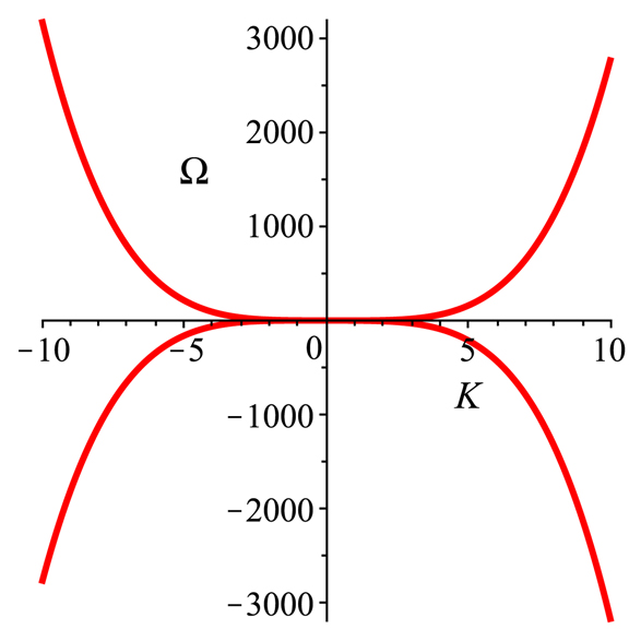
This expression determines the steady-state stability that depends on the the fourth-order dispersion, nonlinear influence, self-steepening effect, higher-order dispersion and wave number. It is clearly seen that the value of frequency $Ω$ is real for all values of K and hence the steady state is stable against small perturbations. Figure 1 shows the graph of dispersion relation.

Figure 1.The dispersion relation Ω = Ω(K) between frequency $Ω$ and wave number K given in (64).

6　Results and discussion

The implemented mathematical tools in terms of the improved projective Riccati equations have led to abundant exact solutions for the perturbed FLE model. All derived solutions are entirely new and different than the ones found in the literatures. Comparing the results obtained here with the corresponding results extracted in the previous studies, it is found that all solutions retrieved in [27] by using the sine–Gordon equation integration scheme can be deduced in this work when B = 0. The created traveling wave solutions include various wave structures such as bright soliton, combo dark–bright soliton, singular soliton, combo singular soliton and periodic waves.

To throw light on the dynamical behaviors of cubic–quartic optical solitons and other waves in polarization-preserving fibers, the graphical representations for some of the constructed exact solutions are presented. Wave structures are displayed in 2D and 3D plots by selecting suitable values of the model parameters. Figure 2 illustrates the evolution of soliton solution (21), where the wave profile shows an M-shaped (two-hump) soliton. The graph in Figure 3 demonstrates periodic singular wave of solution (23). Moreover, Figure 4 presents the plot of solution (25) that describes the bright soliton wave. In Figure 5, the graph of solution (28) depicts the structure of periodic bright soliton train. Additionally, it is clear from Figure 6 that the evolution of solution (31) characterizes the profile of W-shaped wave (dark-dark soliton).

Figure 2.The dynamical behavior of solution (21) with the unity value for all parameters except A = 2.

Figure 3.The dynamical behavior of solution (23) with the unity value for all parameters except b = −1, A = 2, B = i.

Figure 4.The dynamical behavior of solution (25) with the unity value for all parameters except b = −1, B = 2.

Figure 5.The dynamical behavior of solution (28) with the unity value for all parameters except A = i, B = 2i.

Figure 6.The dynamical behavior of solution (31) with the unity value for all parameters except b = −1, B = 0.

7　Conclusion

The present work focused on investigating distinct forms of exact solutions for cubic–quartic Fokas–Lenells equation with Hamiltonian perturbation terms in polarization-preserving fibers. The study is carried out with the aid of the improved projective Riccati equations. The implemented approach enables us to find different wave structures including bright soliton, combo dark–bright soliton, singular soliton and combo singular soliton. Besides, the periodic singular waves are also recovered as a byproduct of executing solution method. The behaviors of some derived solutions are illustrated graphically to pave the way for understanding the physics of the model. Further to this, the stability of the retrieved solutions have been diagnosed by utilizing the linear stability analysis. The modulation instability of the perturbed FLE is discussed and confirms that all extracted solutions are stable. Overall, the proposed algorithm is rich in various solutions which are entirely new and can be exploited in the physical and engineering applications of fiber optics.

References

[1] G.P. Agrawal. Nonlinear fiber optics. Nonlinear Science at the Dawn of the 21st Century, 195-211(2000).

[2] C. De Angelis. Nonlinear optics. Front. Photonics, 1, 628215(2021).

[3] W. Liu, L. Pang, H. Han, M. Liu, M. Lei, S. Fang, H. Teng, Z. Wei. Tungsten disulfide saturable absorbers for 67 fs mode-locked erbium-doped fiber lasers. Opt. Express, 25, 2950-2959(2017).

[4] W. Liu, L. Pang, H. Han, K. Bi, M. Lei, Z. Wei. Tungsten disulphide for ultrashort pulse generation in all-fiber lasers. Nanoscale, 9, 5806-5811(2017).

[5] W. Liu, Y.-N. Zhu, M. Liu, B. Wen, S. Fang, H. Teng, M. Lei, L.-M. Liu, Z. Wei. Optical properties and applications for MoS 2-Sb 2 Te 3-MoS 2 heterostructure materials. Photonics Res., 6, 220-227(2018).

[6] X. Meng, J. Li, Y. Guo, Y. Liu, S. Li, H. Guo, W. Bi, H. Lu, T. Cheng. Experimental study on a high-sensitivity optical fiber sensor in wide-range refractive index detection. JOSA B, 37, 3063-3067(2020).

[7] H. Triki, A.-M. Wazwaz. Combined optical solitary waves of the Fokas–Lenells equation. Waves Random Complex Media, 27, 587-593(2017).

[8] H. Triki, A.-M. Wazwaz. New types of chirped soliton solutions for the Fokas–Lenells equation. Int. J. Numer. Methods Heat Fluid Flow, 27, 1596-1601(2017).

[9] A. Biswas, M. Ekici, A. Sonmezoglu, R.T. Alqahtani. Optical soliton perturbation with full nonlinearity for Fokas–Lenells equation. Optik, 165, 29-34(2018).

[10] A.J.M. Jawad, A. Biswas, Q. Zhou, S.P. Moshokoa, M. Belic. Optical soliton perturbation of Fokas–Lenells equation with two integration schemes. Optik, 165, 111-116(2018).

[11] A. Biswas, H. Rezazadeh, M. Mirzazadeh, M. Eslami, M. Ekici, Q. Zhou, S.P. Moshokoa, M. Belic. Optical soliton perturbation with Fokas–Lenells equation using three exotic and efficient integration schemes. Optik, 165, 288-294(2018).

[12] A. Biswas. Chirp-free bright optical soliton perturbation with Fokas–Lenells equation by traveling wave hypothesis and semi-inverse variational principle. Optik, 170, 431-435(2018).

[13] A. Aljohani, E. El-Zahar, A. Ebaid, M. Ekici, A. Biswas. Optical soliton perturbation with Fokas–Lenells model by Riccati equation approach. Optik, 172, 741-745(2018).

[14] M. Osman, B. Ghanbari. New optical solitary wave solutions of Fokas–Lenells equation in presence of perturbation terms by a novel approach. Optik, 175, 328-333(2018).

[15] E. Krishnan, A. Biswas, Q. Zhou, M. Alfiras. Optical soliton perturbation with Fokas–Lenells equation by mapping methods. Optik, 178, 104-110(2019).

[16] M. Arshad, D. Lu, M.-U. Rehman, I. Ahmed, A.M. Sultan. Optical solitary wave and elliptic function solutions of Fokas–Lenells equation in presence of perturbation terms and its modulation instability. Phys. Scr., 94, 105202(2019).

[17] O. González-Gaxiola, A. Biswas, M.R. Belic. Optical soliton perturbation of Fokas–Lenells equation by the Laplace-Adomian decomposition algorithm. J. Eur. Opt. Soc. Rapid Publ., 15, 13(2019).

[18] K. Al-Ghafri, E. Krishnan, A. Biswas. Chirped optical soliton perturbation of Fokas–Lenells equation with full nonlinearity. Adv. Differ. Equ., 2020, 1-12(2020).

[19] O. González-Gaxiola, A. Biswas, F. Mallawi, M.R. Belic. Cubic-quartic bright optical solitons with improved Adomian decomposition method. J. Adv. Res., 21, 161-167(2020).

[20] G. Genc, M. Ekici, A. Biswas, M.R. Belic. Cubic-quartic optical solitons with Kudryashov’s law of refractive index by F-expansions schemes. Results Phys, 18, 103273(2020).

[21] Y. Yldrm, A. Biswas, A.H. Kara, M. Ekici, A.K. Alzahrani, M.R. Belic. Cubic–quartic optical soliton perturbation and conservation laws with generalized Kudryashov’s form of refractive index. J. Opt., 50, 354-360(2021).

[22] E.M. Zayed, T.A. Nofal, M.E. Alngar, M.M. El-Horbaty. Cubic-quartic optical soliton perturbation in polarization-preserving fibers with complex Ginzburg-Landau equation having five nonlinear refractive index structures. Optik, 231, 166381(2021).

[23] S. Kumar, S. Malik. Cubic-quartic optical solitons with Kudryashov’s law of refractive index by Lie symmetry analysis. Optik, 242, 167308(2021).

[24] E.M. Zayed, K.A. Gepreel, M.E. Alngar, A. Biswas, A. Dakova, M. Ekici, H.M. Alshehri, M.R. Belic. Cubic–quartic solitons for twin-core couplers in optical metamaterials. Optik, 245, 167632(2021).

[25] E.M. Zayed, M.E. Alngar, A. Biswas, Y. Yldrm, S. Khan, A.K. Alzahrani, M.R. Belic. Cubic–quartic optical soliton perturbation in polarization-preserving fibers with Fokas–Lenells equation. Optik, 234, 166543(2021).

[26] A. Biswas, A. Dakova, S. Khan, M. Ekici, L. Moraru, M. Belic. Cubic-quartic optical soliton perturbation with Fokas–Lenells equation by semi-inverse variation. Semicond. Phys. Quantum Electron. Optoelectron., 24, 431-435(2021).

[27] Y. Yıldırım, A. Biswas, A. Dakova, S. Khan, S.P. Moshokoa, A.K. Alzahrani, M.R. Belic. Cubic-quartic optical soliton perturbation with Fokas–Lenells equation by sine–Gordon equation approach. Results Phys, 26, 104409(2021).

[28] K. Al-Ghafri, E. Krishnan, A. Biswas, M. Ekici. Optical solitons having anti-cubic nonlinearity with a couple of exotic integration schemes. Optik, 172, 794-800(2018).

[29] K.K. Al-Kalbani, K. Al-Ghafri, E. Krishnan, A. Biswas. Solitons and modulation instability of the perturbed Gerdjikov-Ivanov equation with spatio-temporal dispersion. Chaos Solitons Fractals, 153(2021).