Quantum state tomography (QST) is a standard process of reconstructing quantum information of an unknown quantum state through measurements of its copies. QST is used to verify state preparation, examine state properties such as correlations, and calibrate experimental systems. It is a crucial part of almost all aspects of experimental quantum information processing, including quantum computing, quantum metrology, and quantum communication.1^–6

As an analog of the “imaging” technique in quantum settings, QST is born to be a data science problem. Given limited copies of an unknown state ρ, we can extract its information via QST. QST is essentially an inverse problem, and such information recovering tasks are well suited to machine learning. Quantum learning theory indicates that Θ(22n/ε2) copies of ρ are necessary and sufficient to learn ρ up to trace distance ϵ.7 Although the tremendous resource requirement makes full-state QST impractical for large-scale systems, several weaker quantum learning models (e.g., probably approximately correct learning,8 online learning,9 and shadow tomography10^,11) can exponentially reduce the computational resource for learning some 2-outcome measurement expectation values or “shadows.”

An artificial neural network (NN), a powerful algorithm in machine learning to fit a specific function, has been widely used for solving quantum information problems, such as quantum optimal control,12^,13 quantum maximum entropy estimation,14 and Hamiltonian reconstruction.15 NNs have also been widely applied for QST applications, such as efficiently recovering the information of local-Hamiltonian ground states from local measurements,16 performing tomography on highly entangled state with large system size,17 mitigating the state preparation and measurement (SPAM) errors in experiments,18 and improving the state fidelity.19^,20 Generative models with NNs can also perform QST with dramatically lower costs.21^,22

In this work, we demonstrate QST with an optical NN (ONN). Several optical implementations for realizing fully connected NN hardware have been proposed and demonstrated recently.23^–28 Optical computing takes advantage of the bosonic wave nature of light: superposition and interference give rise to its intrinsic parallel computing ability. Meanwhile, light is the fastest information carrier in nature. ONN is promising for next-generation artificial intelligence hardware, which provides high energy efficiency, low cross-talk, light-speed processing, and massive parallelism. As compared with the electronic version, ONNs are ideal for dealing with visual signals and information that are naturally generated and coded in light, such as image recognition and vehicular automation. However, most ONN demonstrations are still restricted to linear computation only due to the lack of suitable nonlinearity at a low light level for a large amount of optical neurons.25^–27 Without nonlinear activation functions, ONN is always equivalent to a single-layer structure that cannot be applied for “real” deep machine learning. This problem had not been solved until most recently optical nonlinearity based on electromagnetically induced transparency (EIT),28^,29 phase-change materials,30 and saturated absorption31^,32 was implemented to realize artificial optical neurons for ONNs.

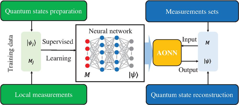
Figure 1 illustrates a general scheme of ONN-QST. First, we collect the training data set from a known quantum state {|ψj⟩} and the corresponding local measurements {Mj}. Second, we train NNs under supervised learning with some nonlinear activation functions in their hidden neurons to obtain the optimal network parameters. Third, we take the trained network parameters to configure the ONN and perform some fine adjustments to optimize the hardware performance. Last, we feed measurement data sets to the trained ONN to reconstruct unknown quantum states. To validate this scheme, in the following sections, we start with a general discussion of QST with the computer-simulated NN and then describe our ONN experimental approach.

We consider a general n-qubit space with Pauli operators (removed the all identity terms) defined as P={σi1(1)⊗⋯⊗σin(n)|σik(k)∈P,∑k=1nik≠0},(1)where P={σ0=I,σ1=X,σ2=Y,σ3=Z}. Every term in P is specified by its index (i1,i2,⋯,in). Measuring every element in P performs a QST for any n-qubit quantum state ρ. For instance, when n=1, we need to measure all three Paulis X,Y,Z for QST. Clearly, the cardinality of P grows exponentially with n. When ρ is a pure state, one may use techniques to reduce the number of measurements for n>1. Compressed sensing is an efficient technique for recovering low-rank quantum states from randomly sampled Pauli operators.33^,34

When ρ is a pure state, it can be written as |ψ⟩=∑k=12nak|ϕk⟩,(2)where {|ϕk⟩} are the computational basis, and the amplitudes ak∈C are normalized [i.e., ∑k=12n(ak,r2+ak,im2)=1, where ak,r∈R and ak,im∈R are the real and imaginary parts of ak, respectively].

The measurement expectation values P are c→=tr(ρ·P)=(tr(ρP1),tr(ρP2),⋯,tr(ρP4n−1)). For a single-qubit pure state α|0⟩+β|1⟩, its density matrix can be expressed as ρ=12(1+c→·σ→),(3)where σ→={X,Y,Z} and c→=(tr(ρX),tr(ρY),tr(ρZ))≡(⟨X⟩,⟨Y⟩,⟨Z⟩).

In compressed sensing, one needs to randomly sample a set Pm={P1,⋯,Pm} of m Pauli operators from P, then use c→=tr(ρ·Pm)=(tr(ρP1),tr(ρP2),⋯,tr(ρPm)) to recover the unknown state ρ, more precisely, the parameters of ρ. This can be regarded as a regression problem to estimate the function between c→ and the parameters of ρ (e.g., ak,r and ak,im).

NNs are excellent tools for solving regression problems. When using NNs for QST, the expectation values c→ from random-sampled Pm are inputs to the network, and state parameters (ak,r, ak,im) are the outputs. Compared with compressed sensing, the NN for QST can be significantly faster when processing many data points. Once the NN is well-trained, it can produce reliable unseen results within an instance, while one needs to solve a convex optimization problem for each data point when applying compressed sensing. Note that both NN-QST and compressed sensing use much fewer measurement settings than the standard method. Without loss of generality, we use the simplest type of NNs in this paper—fully connected feed-forward NNs. The neurons between the nearest layers are fully connected, and the information only passes forward while training. The supervised training process is to compare the ideal outputs (ak,r,ak,im) with current NN outputs and update parameters embedded in the NN to minimize their difference.

We numerically trained computer-based NNs nonlinear activation functions for 1-qubit, 2-qubit, and 3-qubit QST. For the 1-qubit system, the number of sampled operators m∈[1,2,3]; for the 2-qubit system, the number of sampled operators m∈[6,8,10,12]; and for the 3-qubit system, m∈[20,25,30,35,40]. Plainly, m equals the number of input neurons, and n decides the number of output neurons. For each m, three sets of Pauli operators have been sampled and tested. Figure 2 plots the average fidelities (green bars) of both cases as functions of the number of randomly sampled Paulis. For the single-qubit system, the fidelity reaches 99.99% with three Paulis [Fig. 2(a)]. For the 2-qubit system, the fidelity reaches 99.9% with 10 randomly sampled Paulis [Fig. 2(b)]. For the 3-qubit system, a fidelity of higher than 99.9% requires more than 35 randomly sampled Paulis [Fig. 2(c)]. Details of training can be found in Sec. S1 in the Supplemental Materials.

Theoretically, a pure state ρ uniquely determined among all states (UDA) for measuring a set of operators F means that there is no other state, pure or mixed, that has the same expectation values while measuring F.35 In Ref. 36, the authors discovered two sets of Pauli operators, P2−UDA and P3−UDA, that are UDA for all 2-qubit and 3-qubit pure states, respectively (see Sec. S2 in the Supplemental Materials for the particular sets P2−UDA and P3−UDA). Namely, they are special cases of Pauli operator sets that the map between expectation values and the measured state ρ is bijective. Similarly, we apply NNs for these two sets of UDA operators and obtain the prediction fidelities of 99.9% for the 2-qubit case and 99.3% for the 3-qubit case (red triangles in Fig. 2).

We remark that our UDA scheme is not readily scalable for larger systems. However, there exist protocols with better scalability, e.g., compressed sensing,33 shadow tomography,10^,11 where NNs can also be naturally used. In addition, our NN-based scheme can be adapted to quantum tomography in the optical system by taking physical constraints into account, which we will discuss in the next section.

In this first proof-of-principle experimental demonstration, we implement the single-qubit space with light polarizations, i.e., horizontal polarization |H⟩=|0⟩ and vertical polarization |V⟩=|1⟩. Instead of making a full QST, here we focus our task to determine the phase parameter of a pure state |ψ⟩=12(|H⟩+eiθ|V⟩). The experimental ONN-QST setup is displayed in Fig. 3. In conventional QST, an arbitrary polarization state can be reconstructed by measuring the expectation values of the three Pauli operators. Figure 3(a) illustrates such an optical measurement setup. A laser beam passes through a polarization beam splitter (PBS1) and becomes horizontally polarized (|H⟩). The target state |ψ⟩=12(|H⟩+eiθ|V⟩) is prepared by letting this horizontally polarized light pass through a half-wave plate (HWP1) and a quarter-wave plate (QWP1). The expectation values ⟨X⟩, ⟨Y⟩, and ⟨Z⟩ are obtained by sending the light polarization qubit state to the measurement units II, III, and IV shown in Fig. 3(a). To determine ⟨Z⟩, we send the polarization qubit directly to PBS2 which projects |H⟩ and |V⟩ into two photodetectors in the measurement unit III. The normalized differential output from these two photodetectors gives the value ⟨Z⟩. The same setup can also be used to determine ⟨X⟩ or ⟨Y⟩ by placing HWP2 or QWP2 before PBS2 as shown in II or IV, respectively (see Sec. S3 in the Supplemental Materials for details).

We obtain a data set {Mi}={|ϕi⟩:1−⟨X⟩i,1−⟨Y⟩i,1−⟨Z⟩i} by varying the phase θ∈[0,π/2] in the qubit state |ψ⟩=12(|H⟩+eiθ|V⟩) and use them to train our ONN in Fig. 3(b). The ONN comprises an input layer of three neurons, a hidden layer of 20 neurons, and a single-neuron output layer.28^,29Figure 3(b) shows the optical layout of the ONN, and its network structure diagram is displayed in Fig. 3(c). The three coupling laser beams in the optical input layer are generated by a spatial light modulator (SLM1) in Fig. 3(b), lenses L2 and L3, and an aperture, as shown in unit I of Fig. 3(b). The SLM1 is divided into three parts and each part is encoded with the sine phase pattern mπsin[(2π/Tmj)j+(2π/Tmk)k], where m is the modulation depth, Tmj and Tmk are the period of modulation along x and y directions, and j and k are the pixel number along the x and y directions. The sine phase encoded on SLM1 modulates the beams into separated beams at the focal plane of lens L2. The aperture behaves as a filter to keep the zero-order beam, whose intensity is determined by the modulation depth m. Thus, the intensity of the three beams is changed according to the input. The focal beams pass through lens L3 and are collimated and incident to the SLM2. These weighted beams, as the input vector, are incident on SLM2, which diffracts each beam into 20 directions with designed weights (see Sec. S4 in the Supplemental Materials for the algorithm to calculate the pattern encoded on SLM2). A Fourier lens L4 performs linear summation for the beams diffracted into the same direction and forms 20 spots on its front focal plane. Thus, the combination of SLM2 and L4 completes the first linear operation W1 and generates the input to the hidden layer. We then image these 20 spots with lenses L5 and L6 to laser-cooled Rb85 atoms in a two-dimensional magneto-optical trap (MOT),37^,38 where these 20-spot coupling beam patterns spatially modulate the transparency of the atomic medium through EIT.39^,40 Another relatively weak collimated probe beam counterpropagates through the MOT, and its spatial transmission is nonlinearly controlled by the 20-spot coupling beam pattern. Here the nonlinear optical activation functions are realized with EIT in cold atoms. The equation of nonlinear activation functions is as follows: Ipout=f(Ic)=Ipine−OD4γ12γ13Ωc2+4γ12γ13,(4)where Ipin is the power of the input probe beam. Ωc is the Rabi frequency of the coupling beam, and Ωc2 is proportional to coupling beam intensity Ic. Here, γ13=2π×3MHz is fixed and determined by the spontaneous emission of the excited state |3⟩. The ground-state dephasing rate γ12 can be engineered by applying an external magnetic field. OD is the atomic optical depth on the probe transition.

The image of the probe beam transmission pattern by lenses L6 and L8 becomes the output of the 20 hidden neurons. SLM3 and Fourier lens L9 perform the second linear matrix operation W2, and a camera records the output. The technical details of our ONN are described in Refs. 28 and 29.

In this work, because we encode trained NN model and input data into the power of beams, the ONN can only handle positive values: input, output, linear matrix elements, and input/output of nonlinear activation functions are all positive values.28^,29 Meanwhile, the EIT optical nonlinear activation functions are increasing and convex. The lack of negative values in the NN limits its ability. Therefore the ONN is only able to perform regression tasks on increasing and convex functions. To match the ONN constraints, we perform a transform to the input variable, e.g., ⟨X⟩ to 1−⟨X⟩, so that all input values to the ONN nodes are positive. We add these conditions to NN to simulate the ONN performance. The optimizer we use is Adam.41 We find that this specific ONN fails to describe the whole range of nonmonotonic functions. For the first proof-of-principle experimental demonstration, we will only apply the ONN for single-qubit QST with phase θ within [0,π/2]. It is surprising that such a positive-valued ONN is still able to perform some types of QST.

To train the ONN, we prepared the training data set {Mi} from 23 phase values from a uniform distribution θj∼U(0,π/2), corresponding to the optical polarization states {ρj=N(|ϕj⟩⟨ϕj|)}. Here, N is the noise channel in experiments, and measures the Pauli expectation values ⟨X⟩, ⟨Y⟩, ⟨Z⟩. In a similar way, we prepare a test set with 32 independent data samples.

In addition to optical quantum states, we sample data from the IBM quantum (IBMQ) computer ibmq_ourense,42 and implement the same ONN training for comparison. The quantum circuit to prepare |ψ⟩=(|H⟩+eiθ|V⟩)/2 is the initial state |H⟩ going through a Hadamard gate and then going through an RZ rotation gate. On ibmq_ourense, we uniformly sample 158 data points as the training set; 50 data points as the test set. Experimental optical quantum state and IBMQ tomography data are used to train two NNs. Details of training ONN can be found in Sec. S5 in the Supplemental Materials.

Figure 4 shows the ONN state construction results using NN models trained by the ONN-QST training set and the IBMQ computer training set separately. The theoretical value is calculated from ⟨X⟩ directly. With the ONN system set up for the training results, we sent a set of the input vectors to the system. The examples of the real and imaginary parts of the density matrix are shown in Fig. 4(a). The experimentally measured state example is predicted by the ONN QST training model. The example input vector for the ONN model is (⟨X⟩,⟨Y⟩,⟨Z⟩)=(0.440,0.898,0) and the experimental ONN predicted state is θ=1.195 and ρ=(0.50.1852−0.46457i0.1852+0.46457i0.5) which is close to the theoretical value θ=1.1152 and NN predicted value θ=1.1532. The state is also marked with a yellow triangle in Fig. 4(b1). The experimental results are shown in Fig. 4(b). The theoretical value, NN predicted value, and experimental ONN predicted value agree with both optics data training [Fig. 4(b1) shows] and IBMQ data training [Fig. 4(b2)shows]. The theoretical value, NN prediction value, and ONN predicted value are consistent in both cases. The results suggest that our positive-valued ONN with EIT nonlinear activation functions is capable of qubit QST.

While most demonstrations of ONNs took classification tasks to verify their feasibility,26^,27^,30 we performed the first regression task, i.e., ONN-QST. To accomplish regression tasks, the nonlinear function is essential as long as the relation between the input vector and output vector cannot be expressed linearly. The tunable EIT nonlinear optical activation functions in our ONN offer opportunities for performing regression tasks with convex and increasing/decreasing functions. Although our ONN has some certain limitations that the linear operation matrix elements are all positive valued, it has the potential to do large-size QST with restrictions.

Further, ONN can play a positive role in the noisy intermediate-scale quantum (NISQ) era. In NISQ algorithms, one usually only needs to reconstruct some reduced density matrix and extract the required local information instead of characterizing the whole system through a full-state tomography. ONN-QST can serve as an efficient subroutine to speed up this process. For example, within each Trotter step of the quantum imaginary time evolution,43^,44 we can train an ONN to reconstruct the reduced density matrix of some neighboring qubits, then use this information to determine the direction of the next step.

To perform QST for a higher dimensional space requires more active neurons. Our theoretical simulation shows 10 and 30 inputs are needed for the 2-qubit and 3-qubit cases, respectively. However, while the number of optical neurons is not a limiting factor in our current experimental setup, the ONN input/output and matrix weights are all positive-valued. Meanwhile, the nonlinear activation functions we implemented are increasing and convex, and it is impossible to conduct the regression task of nonmonotonic functions experimentally. These physical limitations limit us to performing more complicated QST. We believe the next generation of complex-valued ONNs with data encoded in both light amplitude and phase will be more powerful. The future development of complex-valued ONNs may enable large-size QST and more applications.

Optical quantum networks45 have been brought to the fore by the reduced decoherence and high speed of photons. Recently, apart from generating optical quantum states46 and optical quantum communication over a long distance,47 multiple state-of-the-art experiments on optical quantum interfaces to store48 and distribute entanglements49^,50 have been exhibited. Among all of these, QST is essential for characterizing the generation and preservation of quantum states and has the potential to verify the entanglement distributed across the whole network. We believe that our optical setup of integrated ONN-QST will shed light on replenishing the optical quantum network with one more brick.

Ying Zuo received her BSc degree from the University of Science and Technology of China, Hefei, Anhui, China, in 2017. Upon completion of this work, she is a PhD candidate at the Hong Kong University of Science and Technology, supervised by Prof. Shengwang Du and Prof. Bei Zeng. Her research interests focus on optical computing and quantum optics.

Chenfeng Cao received his BSc degree from the University of Chinese Academy of Sciences, Beijing, China, in 2019. Currently, he is a PhD candidate supervised by Prof. Bei Zeng at the Hong Kong University of Science and Technology. His research interests lie in quantum information and quantum computing.

Ningping Cao received her PhD from the University of Guelph, Ontario, Canada, in 2021. Currently, she is a postdoc fellow at the Institute of Quantum Computing (IQC), University of Waterloo, Ontario, Canada. She is interested in a wide range of topics in quantum information and quantum computation.

Xuanying Lai received her BS degree from East China Normal University in 2020. Currently, she is pursuing her PhD under the supervision of Prof. Shengwang Du in the Department of Physics at the University of Texas at Dallas. Her research focus is quantum optics.

Bei Zeng is a professor at the Hong Kong University of Science and Technology. Her research focus is on the design of quantum error-correcting codes with nice properties that are suitable for high rate quantum information transmission through practical physical channels, and reliable quantum computation with high noise tolerance and low resource requirement. She is a fellow of APS.

Shengwang Du, currently a professor of physics at the University of Texas at Dallas since 2021, worked at the Hong Kong University of Science and Technology from 2008 to 2020. His group is exploring fundamentals in the field of atomic, molecular, and optical (AMO) physics, and their applications. His current research activities include quantum networks, all-ONNs, and applied optical microscopy. He is a fellow of both APS and Optica (formerly OSA).