Phase-unwrapping algorithm combined with wavelet transform and Hilbert transform in self-mixing interference for individual microscale particle detection

Yu Zhao; Jiawei Li; Menglei Zhang; Yangyang Zhao; Jianglin Zou; Tao Chen

doi:10.3788/COL202321.041204

Abstract

The self-mixing interferometry (SMI) technique is an emerging sensing technology in microscale particle classification. However, due to the nature of the SMI effect raised by a microscattering particle, the signal analysis suffers from many problems compared with a macro target, such as lower signal-to-noise ratio (SNR), short transit time, and time-varying modulation strength. Therefore, the particle sizing measurement resolution is much lower than the one in typical displacement measurements. To solve these problems, in this paper, first, a theoretical model of the phase variation of a single-particle SMI signal burst is demonstrated in detail. The relationship between the phase variation and the particle size is investigated, which predicts that phase observation could be another alternative for particle detection. Second, combined with continuous wavelet transform and Hilbert transform, a novel phase-unwrapping algorithm is proposed. This algorithm can implement not only efficient individual burst extraction from the noisy raw signal, but also precise phase calculation for particle sizing. The measurement shows good accuracy over a range from 100 nm to 6 μm with our algorithm, proving that our algorithm enables a simple and reliable quantitative particle characteristics retrieval and analysis methodology for microscale particle detection in biomedical or laser manufacturing fields.

Keywords

continuous wavelet transform Hilbert transform laser processing particle detection self-mixing interferometry

1. Introduction

Thanks to its intrinsic advantages of high simplicity, low cost, and the same resolution as that of the typical Michelson interferometer, self-mixing interferometry (SMI), also named optical feedback interferometry (OFI), has been well-established in various metrology applications, and not only in traditional industrial fields, such as vibration displacement, velocimetry, and absolute distance finding^[1–5], but also in laser welding monitoring, particle sizing, or label-free biomedical sensing^[6–8].

Currently, SMI has attracted much attention in microparticle detection in chemical and biomedical fields, since this simple technique is very suitable for an integrated platform with microfluidic chip and other devices like fuel nozzles^[9–14]. Particularly, SMI can be a promising candidate for real-time single-particle detection for small dosage agent experiments in flow cytometry or particle mixing. Moreira et al., for the first time, observed the presence of single submicroscale particles in a 320 µm channel using SMI technology. They applied a simple bandpass filter to visualize the particle bursts in the noisy raw signal and measured the single-particle velocity by fast Fourier transform (FFT)^[15]. Contreras et al. managed to classify the single polystyrene sphere size for a higher signal-to-noise ratio (SNR). They developed a novel SMI scheme with edge-filter-enhanced self-mixing interferometry (ESMI)^[16], and they approached around 2 orders of magnitude, even at a 10 m operating distance. Zhao et al. presented a fringe counting method for single-microparticle sizing based on the Hilbert transform (HT)^[17]; the resolution was still a half wavelength. Unlike the continuous SMI signal from a bulk translating target, particle-induced signals represent a discrete waveform burst. This innovative topic is still challenging: the SMI signal is lower in amplitude and temporally discrete on a millisecond scale. The noises from the measurement environment can significantly reduce SNR and spoil the performance of the sensor system. The resolution in this specific scenario is limited to a basic half wavelength; what is more, the retrieved fringe pattern still presents the signal ambiguity in the waveform edge, where some fringes are missing.

Besides measuring temporal signal waveform fringe number^[18] and frequency spectral width^[7], novel precise alternatives for particle detection are still required. As a kind of phase observation tool, the phase-unwrapping method (PUM) has been exhaustively studied in SMI sensor systems^[19–27], and the spatial resolution even can reach $λ / 67$ ^[28]. This processing method normally involves two steps: the first step is phase retrieval, and the second step is to estimate the feedback factor and linewidth enhancement factor for phase profile correction and displacement reconstruction. Apart from the typical vibration or displacement measurements, SMI signal phase assessment was also employed in 2D scanning and surface profile mapping. Lacot et al. proposed a new low-noise and phase-sensitive detection scheme for scattering-type scanning near-field optical microscopy (sSNOM). They successfully implemented high-resolution phase imaging of silicon-on-insulator (SOI) optical waveguides^[29]. Considering the high resolution, PUM can be a good candidate for particle detection; however, there appears to be no related literature existing on this topic.

Sign up for Chinese Optics Letters TOC. Get the latest issue of Chinese Optics Letters delivered right to you！Sign up now

The paper is organized as follows. First, a theoretical framework of SMI effect in the presence of a translating particle is demonstrated, and during the particle passage, the dependence of SMI signal phase variation on particle size is investigated. Second, for effective noise elimination and phase retrieval, continuous wavelet transform (CWT) is directly applied to the original SMI signal. And then a simple HT-based PUM is employed for phase calculation and unwrapping, with the resultant phase variation corresponding to single particle extraction. Finally, using a 532 nm solid-state laser SMI system, signal bursts induced by different-sized polymer beads are acquired and processed by our algorithm, and the measured phase variation values are compared with the simulation results.

2. Theory

When a laser shoots a beam onto a remote target and a portion of the backreflected or backscattered light re-enters the laser cavity, the interaction between the coupled feedback light and the emitting laser field evokes a laser output power fluctuation. The modulated laser output power $P (t)$ in the presence of self-mixing effect can be expressed by Eq. (1), $P (t) = P_{0} [1 + m (t) \cos ϕ] .$ (1)

$P_{0}$ is the original laser output power, and $m$ is the modulation index, which depends on the scattering intensity. $ϕ$ denotes the phase in the presence of the SMI effect, whose value can be calculated by the well-known excess phase equation^[30], $ϕ_{0} = ϕ + C (\cos ϕ + \arctan α) .$ (2)

$ϕ_{0}$ is the initial phase without feedback effect, $C$ is the feedback coefficient, determining the feedback strength, and $α$ is the linewidth enhancement factor^[31]. But when the target is a microscale moving particle, the backward scattering light acts as the feedback light, and the $C$ value is typically smaller than 1^[11]. The SMI system then operates in a weak feedback region, and the phase hysteresis can be negligible. Due to the well-known Doppler effect, the instant phase $ϕ$ value can be approximately given by^[32,33] $ϕ (t) = 2 π f_{d} \cdot t .$ (3) $f_{d}$ is the Doppler frequency that depends on the particle velocity and the incidence angle between the laser axis and the particle translation direction $θ_{inc}$ , $f_{d} = \frac{2 V \cdot \cos θ_{inc}}{λ} .$ (4)

Considering that the incident laser beam exhibits a Gaussian spatial intensity profile, and the scattering intensity properties of the particle are also strongly dependent on its position during the flight, both phenomena influence the modulation index $m$ value. Thus, we assume the $m$ value varies as a Gaussian function during the particle flowing inside the measurement volume, and the signal expression can be rewritten by Eq. (5)^[17], $P (t) = P_{0} (1 + m \cdot \cos f_{d} \cdot t) \exp [- \frac{{(t - t_{0})}^{2}}{2 τ^{2}}] .$ (5)

$τ$ is the particle passage period inside the measurable region of the sensor system, whose dimension $M$ can be simplified as the combination of laser spot size $K$ and the particle diameter $D$ . When $t = t_{0}$ , the laser beam shoots onto the particle or cell center perpendicularly, and the particle center passes the light axis^[18], $τ = \frac{M}{V \sin θ} = \frac{K + D}{V \sin θ} .$ (6)

During the signal burst period $τ$ , the total phase variation $Φ$ is given by Eq. (7), as a linear function of $τ$ , without dependence on velocity, $Φ = 2 π f_{d} \cdot τ .$ (7)

From Eqs. (6) and (7), the phase variation $Φ$ can be derived as a proportional function of the detectable region distance $M$ by Eq. (8). $K$ and $D$ are fixed in the given experiment; neither of them depends on the velocity, $Φ = \frac{4 π}{λ} \cdot \frac{\cos θ}{\sin θ} \cdot M = \frac{4 π}{λ} \cdot \frac{\cos θ}{\sin θ} (K + D) .$ (8)

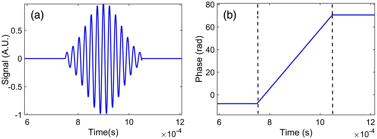
The particle diameter $D$ can be very easily calculated by the given equation, $D = \frac{λ}{4 π} \cdot \frac{\sin θ}{\cos θ} Φ - K .$ (9)

We simulate the signal burst and the phase variation with the parameters in Table 1. The simulation results are shown in Fig. 1. Within the signal burst period (dashed line), the phase increases linearly as Eq. (7). The signal burst region can be exactly distinguished by the phase profile.

Figure 1.Simulated signal from a 5 µm diameter particle. (a) Temporal signal; (b) phase profile.

Parameter	λ	θ_inc	D	K
Value	532 nm	25°	5 µm	1 µm

Table 1. Parameters for Simulation

View all Tables

3. Data Processing Method

According to the above-mentioned section, the particle-induced SMI signal is in a temporally intermittent form during the particle passage. Moreover, the signal burst normally is affected by white Gaussian noise, impulsive noise, and DC pedestal^[34,35]. The signal burst of each particle is ambiguous and merged in the noises, so an efficient method of burst identification and denoising is demanded. The CWT is a well-established method for investigation of time and frequency details of signals whose frequency content varies over time^[23,36,37]. Eventually, this technique performs a correlation between a scaled/shifted wavelet basis and the SMI signal. Because the resultant amplitude corresponding to the uncorrelated and random noise is much lower than that of the desired signal, CWT can implement noise removal in a single step without additive complicated processing.

In this paper, CWT is applied to the SMI signal $Sig (t)$ . Based on CWT principles^[21], the CWT coefficient $W$ of the signal is expressed as follows: $W (u, s) = \frac{1}{\sqrt{s}} \int_{- \infty}^{+ \infty} Sig (t) ψ (\frac{t - u}{s}) d t,$ (10)where $s$ is the scaling factor, describing the time length of single-period wavelet basis, and $u$ is the shifting factor. By changing the $t$ and $u$ values, CWT enables effective SMI signal decomposition into different frequency components.

$ψ$ is the wavelet basis. There are many types of wavelet basis, such as Daubechies (db), Morlet, Coiflets, and Haarhere. Considering the particle-induced frequency modulation signal is sinusoidal-like in Eq. (5), we chose Morlet, whose capability has been proven in SMI measurements^[38], as the wavelet basis in the data processing. The Morlet CWT basis with a frequency $ω_{0}$ in the time domain is defined as follows: $ψ (t) = π^{- 1 / 4} e^{i ω_{0} t} e^{- t^{2} / 2} .$ (11)

The HT can represent a signal in its analytical form over the orthogonal plane and retrieve the phase information very conveniently without modifying the amplitude. So HT is very suitable for phase unwrapping in SMI measurements^[17,19].

The original signal function $f (t)$ can be transformed into a complex analytical form as a combination of a real part $ξ (t)$ and an imaginary part $Θ (t)$ , as in Eq. (12), $f (t) = ξ (t) + j \cdot Θ (t),$ (12)and $Θ (t)$ is calculated by performing a 90° phase shift of the real part by an HT^[17], $Θ (t) = HT [ξ (t)] .$ (13)

Finally, the instant phase $ϕ (t)$ can be calculated using inverse tangent function, $ϕ (t) = \arctan \frac{ξ (t)}{Θ (t)} .$ (14)

After the HT, using a MATLAB-customized phase-unwrapping routine, the realistic phase $Φ$ can be calculated after the unwrapping, $Φ = ϕ (t) + 2 n π,$ (15)where $n$ is an integer, and the value of $n$ is 0, 1, 2, ….

The data processing flow chart is illustrated in Fig. 2. The algorithm involves two steps: first, CWT for raw signal noise elimination and burst retrieval; second, HT for phase estimation and unwrapping function.

Figure 2.Chart diagram of CWT-HT signal processing algorithm for particle-induced SMI signal.

4. Experiment and Results

To validate the simulation and the capability of our algorithm, a series of particle sizing measurements are performed with the setup shown in Fig. 3. We select a compact diode-pumped solid-state laser (DPSS) at 532 nm wavelength (Thorlabs, DJ532-10) as the SMI laser source in the system. Due to the higher ratio of fluorescence-to-photon lifetime, a DPSS SMI configuration has higher sensitivity than the typical laser diode (LD) setup^[39]. The laser is controlled by a laser controller (Thorlabs, ITC4001), and the injection current and the laser package temperature are kept to be 240 mA and $24 ° C \pm 0.1 ° C$ , respectively. The collimated output light is spliced into two beams by a 1:9 beam splitter (BS). One beam path (90%) as a detection path is focalized tightly by an aspherical lens (Thorlabs, CMD240-C) and shot onto the microparticle flux. The laser spot diameter $K$ is around 1 µm, and the incidence angle $θ_{inc}$ is $25 \pm 1 \deg$ . The other beam path (10%) is directed to a fixed gain photodiode detector (Thorlabs, PDF10A2) for SMI signal retrieving. Afterward, the SMI voltage signal is digitized using a fast speed data acquisition card (NI, 6361USB). The sampling frequency and acquisition data number are 500 kHz and $2^{17}$ , respectively. Polystyrene spheres (PSs) in seven different diameters (100, 500, 2, 3, 4, 5, and 6 µm) are employed as the scattering objects, and the particle stream is made by a homemade powder feeder. The dimension coefficients of variation (CVs) of the particles are better than 3%.

Figure 3.Schematic of SMI system.

Thousands of monodispersed signal bursts in different particle sizes are captured and processed by our above-mentioned algorithm. The raw signal burst without processing in 2 µm is denoted by the black line in Fig. 4(a). As the figure shows, the signal burst is merged in the strong noise floor, leading to great difficulty in interference fringe observation. To reduce the noise, we applied both bandpass filter (BPF) and Morlet-based CWT upon the raw signal, respectively. Firstly, we analyze the signal by CWT, and the scalogram of the real part of the CWT coefficient $W$ is then depicted in Fig. 4(b) to visualize both the spatial and temporal components. It can be seen that the maximum $W$ value in light yellow color is located in the temporal range from 21.3 to 23.5 ms, representing the particle flight period inside the laser illumination area, and the frequency is in a limited range from 2 to 4 kHz.

Figure 4.Signal burst of 2 µm PS particle. (a) Raw SMI signal (black), denoised SMI signals by BPF (red) and CWT (blue); (b) scalogram of CWT.

We set the threshold to be 0.2 of the maximum $W$ value and eliminate the signal level under the threshold value. Besides the CWT, we also use a fifth-order Butterworth BPF as reference^[17] for signal denoising. We set the filter cut-off frequency range to be from 2 to 4 kHz, the same as the scalogram shows. The blue line and red line denote the denoised bursts from the CWT and the BPF in Fig. 4(a), respectively. The bursts are added $\pm 0.4 V$ amplitude offset for more convenient observation.

From the figures, it can be seen that even though the BPF can eliminate the noise effectively in the red line, the burst margin regions are still greatly ambiguous. There are some supernumerary noise fluctuations remaining in the dashed line circles, which can be mistaken for extra signal interference fringes. Compared with the BPF, a well-defined impulse waveform corresponding to a single particle can be distinguished easily by CWT (blue line) without margin ambiguity.

Afterward, the denoised signals are processed by the HT-PUM algorithm to calculate the phase profile. As shown in Fig. 5, obviously, both phase profiles present good linear trend as the simulation. However, compared with the one from the BPF, the linear profile CWT bends at the burst period endpoint, which is exactly the same as in the scalogram in Fig. 4(b). The total phase variation from the starting point $t = 21.3 ms$ to the ending point $t = 23.5 ms$ is around 31 rad, which is in good agreement with the calculation from Eq. (8). From the results, we can conclude that even without the scalogram prediction, CWT can precisely extract the signal scope in both time domain and the phase profile regardless of the noise.

Figure 5.Phase profiles of the 2 µm PS particle SMI signal by BPF (red) and CWT (blue).

By using the threshold CWT algorithm, the particle signals in other different particle sizes are also illustrated in Fig. 6, indicating the robustness of denoising ability with CWT.

Figure 6.Signal bursts of the PS particles in different diameters after CWT denoising. (a) 500 nm; (b) 3 µm; (c) 4 µm; (d) 5 µm.

Signal burst retrievals from each particle size are repeated around 30 times; the mean values of the measured phase $Φ$ as a function of the particle diameter (blue marks) and the simulation by Eq. (8) (black line) are depicted in Fig. 7. It should be noted that the measurement results present a good linear profile with respect to the linear fitting (red line), which is expected in simulation. The measurement and simulation results are generally in good agreement over the whole given particle size range, with a slight deviation. The measured laser spot size $K$ value is a little smaller than the simulated one. This can be explained by the uncertain quantities of the measurement value before the particle sizing experiment. The slope of the measurement trend (the red line) is greater than the simulated one; the incident angle deviation is the most credible reason for this phenomenon. Unfortunately, both $K$ and $θ_{inc}$ discrepancies are difficult to avoid in practice.

Figure 7.Phase curve as a function of the particle diameter. The blue circle marks represent the mean values and the standard deviations of the measured value of phase $Φ$ . The black line and red solid line denote the simulation results and the linear fitting.

5. Conclusion

In this work, we present a simple and capable PUM algorithm for single-particle size characterization. CWT and HT are involved for noise elimination, individual particle-induced burst retrieval, and phase calculation. The resultant phase variation corresponding to single-particle modulation is extracted efficiently compared with the typical bandpass filtering. The experimental results showed good linear trend of SMI signal phase variation with the particle size over a practical valuable measurement range from 100 nm to 6 µm, which corresponds to typical living cells and bacteria. The good consistency between the simulation results and measured signals has proven the reliability of our theoretical model and the capability of phase observation method in microparticle detection. Thus, the advantage of the new approach with our CWT-HT-PUM algorithm can be more pronounced for particle sizing in the biomedical and chemical fields. Unlike in displacement or vibration measurements, a piezoelectric translator (PZT) enables ultraprecise target motion on a 0.1 nm scale. In our measurement, the artificial particle diameter cannot be regulated less than 1 µm, and the particle dimension inhomogeneity is inevitable during fabrication. So the minimum particle sizing limitation of our method cannot be validated perfectly for the moment. More experiments with finer particle size deviation could be performed in future.

References

[1] Y. Tan, S. Zhang, Z. Ren, Y. Zhang, S. Zhang. Real-time liquid evaporation rate measurement based on a microchip laser feedback interferometer. Chin. Phys. Lett., 30, 124202(2013).

[2] Z. Zhang, L. Sun, C. Li, Z. Huang. Laser self-mixing interferometry for micro-vibration measurement based on inverse Hilbert transform. Opt. Rev., 27, 90(2020).

[3] P. Qi, J. Cheng, S. Li, Z. Zhang, G. Song, J. Weng, J. Zhong. Experimental observation of differential self-mixing interference signals using a randomly polarized laser: a differential self-mixing interferometry. Opt. Lett., 45, 1858(2020).

[4] S. Donati, M. Norgia. Native signal self-mix interferometer has less than 1-nm noise-equivalent-displacement. Opt. Lett., 46, 1995(2021).

[5] M. Veng, F. Bony, J. Perchoux. Disappearance of fringes in the self-mixing interferometry sensing scheme: impact of the initial laser mode solution. Opt. Lett., 46, 1991(2021).

[6] J. Zou, J. Gong, X. Han, Y. Zhao, Q. Wu. In situ detection of plume particles in intelligent laser welding. Mater. Des., 217, 110633(2022).

[7] C. Wang, K. Kou, J. Yan. Frequency-shifted nano-particle sizing using laser self-mixing interferometry. Laser Phys. Lett., 19, 066202(2022).

[8] Z. Dai, X. Xu, Y. Wang, M. Li, K. Zhou, L. Zhang, Y. Tan. Surface plasmon resonance biosensor with laser heterodyne feedback for highly-sensitive and rapid detection of COVID-19 spike antigen. Biosens. Bioelectron., 206, 114163(2022).

[9] C. Zakian, M. Dickinson, T. King. Dynamic light scattering by using self-mixing interferometry with a laser diode. Appl. Opt., 45, 2240(2006).

[10] K. Otsuka, T. Ohtomo, H. Makino, S. Sudo, J.-Y. Ko. Net motion of an ensemble of many Brownian particles captured with a self-mixing laser. Appl. Phys. Lett., 94, 241117(2009).

[11] Y. Zhao, J. Perchoux, L. Campagnolo, T. Camps, R. Atashkhooei, V. Bardinal. Optical feedback interferometry for microscale-flow sensing study: numerical simulation and experimental validation. Opt. Express, 24, 23849(2016).

[12] H. Wang, J. Shen. Size measurement of nano-particles using self-mixing effect. Chin. Opt. Lett., 6, 871(2008).

[13] J. Zou, Z. Huang, J. Gong, Y. Zhao, Z. Wang, Q. Wu. Characterization of micron-sized particles in the focused laser beam during fiber laser keyhole welding. Opt. Laser Technol., 156, 108463(2022).

[14] J. Zou, Z. Wang, Y. Zhao, X. Han, J. Gong. In situ measurement of particle flow during fiber laser additive manufacturing with powder feeding. Results Phys., 37, 105483(2022).

[15] R. da Costa Moreira, J. Perchoux, Y. Zhao, C. Tronche, F. Jayat, T. Bosch. Single nano-particle flow detection and velocimetry using optical feedback interferometry(2017).

[16] V. Contreras, J. Lönnqvist, J. Toivonen. Detection of single microparticles in airflows by edge-filter enhanced self-mixing interferometry. Opt. Express, 24, 8886(2016).

[17] Y. Zhao, M. Zhang, C. Zhang, W. Yang, T. Chen, J. Perchoux, E. E. Ramírez-Miquet, R. da Costa Moreira. Micro particle sizing using Hilbert transform time domain signal analysis method in self-mixing interferometry. Appl. Sci., 9, 5563(2019).

[18] Y. Zhao, X. Shen, M. Zhang, J. Yu, J. Li, X. Wang, J. Perchoux, R. da Costa Moreira, T. Chen. Self-mixing interferometry-based micro flow cytometry system for label-free cells classification. Appl. Sci., 10, 478(2020).

[19] S. Amin. Implementation of Hilbert transform based high-resolution phase unwrapping method for displacement retrieval using laser self mixing interferometry sensor. Opt. Laser Technol., 149, 107887(2022).

[20] Z. Huang, B. Du, Z. Zhang, Y. Ye, S. He, Z. Li, S. He, X. Hu, D. Li. Compact photothermal self-mixing interferometer for highly sensitive trace detection. Opt. Express, 30, 1021(2022).

[21] D. Li, Q. Li, X. Jin, B. Xu, D. Wang, X. Liu, T. Zhang, Z. Zhang, M. Huang, X. Hu, C. Li, Z. Huang. Quadrature phase detection based on a laser self-mixing interferometer with a wedge for displacement measurement. Measurement, 202, 111888(2022).

[22] Z. Wu, W. Guo, L. Lu, Q. Zhang. Generalized phase unwrapping method that avoids jump errors for fringe projection profilometry. Opt. Express, 29, 27181(2021).

[23] Y. Zhao, B. Zhang, L. Han. Laser self-mixing interference displacement measurement based on VMD and phase unwrapping. Opt. Commun., 456, 124588(2020).

[24] S. Amin, U. Zabit, O. D. Bernal, T. Hussain. High resolution laser self-mixing displacement sensor under large variation in optical feedback and speckle. IEEE Sens. J., 20, 9140(2020).

[25] C. Jiang, X. Wen, S. Yin, Y. Liu. Multiple self-mixing interference based on phase modulation and demodulation for vibration measurement. Appl. Opt., 56, 1006(2017).

[26] Z. Zhang, C. Li, Z. Huang. Vibration measurement based on multiple Hilbert transform for self-mixing interferometry. Opt. Commun., 436, 192(2019).

[27] J.-H. Kim, C.-H. Kim, T.-H. Yun, H.-S. Hong, K.-M. Ho, K.-H. Kim. Joint estimation of self-mixing interferometry parameters and displacement reconstruction based on local normalization. Appl. Opt., 60, 2282(2021).

[28] X. Wan, D. Li, S. Zhang. Quasi-common-path laser feedback interferometry based on frequency shifting and multiplexing. Opt. Lett., 32, 367(2007).

[29] S. Blaize, B. Bérenguier, I. Stéfanon, A. Bruyant, G. Lérondel, P. Royer, O. Hugon, O. Jacquin, E. Lacot. Phase sensitive optical near-field mapping using frequency-shifted laser optical feedback interferometry. Opt. Express, 16, 11718(2008).

[30] T. Taimre, M. Nikolić, K. Bertling, Y. L. Lim, T. Bosch, A. D. Rakić. Laser feedback interferometry: a tutorial on the self-mixing effect for coherent sensing. Adv. Opt. Photonics, 7, 570(2015).

[31] R. Lang, K. Kobayashi. External optical feedback effects on semiconductor injection laser properties. IEEE J. Quantum Electron., 16, 347(1980).

[32] C. Yáñez, F. J. Azcona, S. Royo. Confocal flowmeter based on self-mixing interferometry for real-time velocity profiling of turbid liquids flowing in microcapillaries. Opt. Express, 27, 24340(2019).

[33] Y. Tao, M. Wang, W. Xia. Semiconductor laser self-mixing micro-vibration measuring technology based on Hilbert transform. Opt. Commun., 368, 12(2016).

[34] Z. A. Khan, U. Zabit, O. D. Bernal, T. Hussain. Adaptive estimation and reduction of noises affecting a self-mixing interferometric laser sensor. IEEE Sens. J., 20, 9806(2020).

[35] Y. Zhao, T. Camps, V. Bardinal, J. Perchoux. Optical feedback interferometry based microfluidic sensing: impact of multi-parameters on Doppler spectral properties. Appl. Sci., 9, 3903(2019).

[36] O. D. Bernal, H. C. Seat, U. Zabit, F. Surre, T. Bosch. Robust detection of non-regular interferometric fringes from a self-mixing displacement sensor using bi-wavelet transform. IEEE Sens. J., 16, 7903(2016).

[37] Y. Wei, Y. Wei, W. Huang, Z. Wei, J. Zhang, T. An, X. Wang, H. Xu. Double-path acquisition of pulse wave transit time and heartbeat using self-mixing interferometry. Opt. Commun., 393, 178(2017).

[38] A. Jha, F. J. Azcona, C. Yañez, S. Royo. Extraction of vibration parameters from optical feedback interferometry signals using wavelets. Appl. Opt., 54, 10106(2015).

[39] K. Kou, C. Wang, T. Lian, J. Weng. Fringe slope discrimination in laser self-mixing interferometry using artificial neural network. Opt. Laser Technol., 132, 106499(2020).