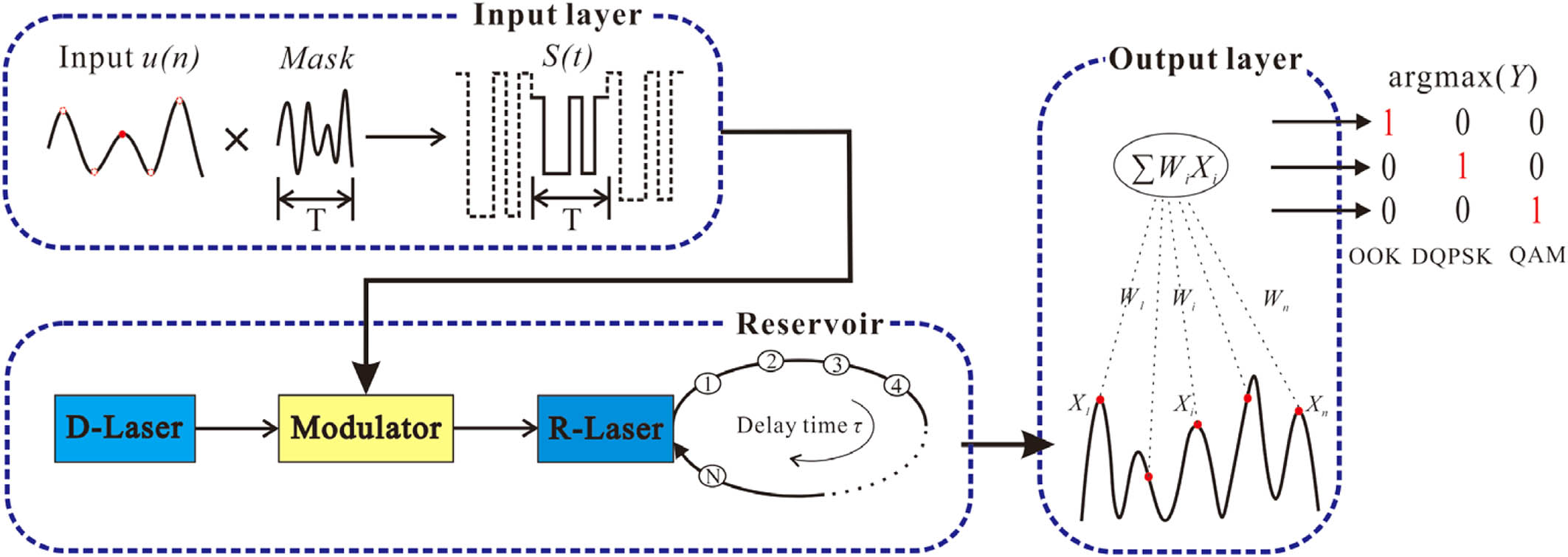
Fig. 1. Schematic of the MFI based on the P-RC with semiconductor lasers. This system consists of three parts: input layer, reservoir, and output layer. The input u(n) is multiplied by a mask with a period of T, and then the resulting stream S(t)=Mask×u(n) is fed into the reservoir through a modulator. The reservoir is a master-slave configuration constructed by a response laser (R-Laser) with a self-delay feedback loop injected by a drive laser (D-Laser). Note that there are N virtual nodes at each interval θ in the feedback loop with a delay time of T. The transient states of the R-Laser Xi are read out for training the connection weights Wi between the reservoir and the output layer. The final output nodes are weighted by the sums of the transient states ∑XiWi.

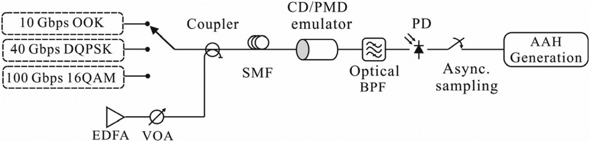
Fig. 2. Sketch of the emulated transmission system for asynchronous amplitude histogram generation. EDFA, erbium-doped fiber amplifier; SMF, single-mode fiber; CD/PMD, chromatic dispersion/polarization mode dispersion; BPF, band-pass filter; PD, photodetector; AAH, asynchronous amplitude histogram.

Fig. 3. Typical asynchronous amplitude histograms for (a1)–(a3) OOK, (b1)–(b3) DQPSK, and (c1)–(c3) QAM formats after propagation through the emulated communication channel. From left to right, each column has an OSNR of 12, 19, and 26 dB, while the corresponding CD and the DGD are fixed at 80 ps/nm and 5 ps, respectively.

Fig. 4. (a) Identification error rate on the total (training and test) sample numbers of the binary mask (black), the six-level mask (blue), and the chaos mask signals (red). (b) Dependence of the identification error rate on the total (training and test) sample numbers at different virtual node sizes of 300 (blue) and 400 (red).

Fig. 5. (a) Bifurcation diagram of the output optical intensity versus the injection strength kinj for kf=0.18, IR=1.3Ith, and Δν=−10  GHz. (b) Identification error rate (ER) at different injection strengths kinj (blue dots), while the red curve is plotted by executing a sliding window averaging to the associated data points.

Fig. 6. (a) Bifurcation diagram of the output optical intensity versus the feedback strength kf for kinj=0.2, IR=1.3Ith, and Δν=−10  GHz. (b) Identification ER at different feedback strengths kf (blue dots), while the red curve is plotted by executing a sliding window averaging to the associated data points.

Fig. 7. (a) Bifurcation diagram of the output optical intensity versus the bias current of the R-Laser IR for kinj=0.2, kf=0.15, and Δν=−10  GHz. (b) Identification ER at different bias currents of the R-Laser IR (blue dots), while the red curve is plotted by executing a sliding window averaging to the associated data points.

Fig. 8. (a) Bifurcation diagram of the output optical intensity versus the frequency detuning Δν between the D-Laser and the R-Laser for kinj=0.2, kf=0.15, and IR=1.25Ith. (b) Identification ER at different frequency detunings Δν (blue dots), while the red curve is plotted by executing a sliding window averaging to the associated data points.

Table 1. Identification Accuracies for Different Modulation Formats Using the MFI Technique Through Our Laser-Based P-RC System^a

Table 2. Identification Accuracies for Different Modulation Formats Using Only the Ridge Regression Algorithm (Without the Reservoir Layer in the System)^a

Table 3. Identification Accuracies for Different Modulation Formats Using the MFI Technique Through the P-RC System with a Typical Noise Value of β=1.5×10−6^a