Fiber-optic communication systems are expected to be capable of adaptively adjusting various transmission parameters such as modulation formats, line rates, and spectrum assignments, based on the varying channel conditions and traffic demands in order to maximize the spectral and energy efficiencies [1–4]. The dynamic variation of transmission parameters imposes new requirements for the optical receivers in such elastic optical networks (EONs). To demodulate the transmission signal at the digital receivers, one must know the type of modulation format. Consequently, correct identification of modulation formats is rather crucial for high-quality communication [5,6].

The feature-based (FB) approach is an effective way to achieve modulation format identification (MFI) [7–11], carried out by using different tools to analyze the associated feature parameters from transmission signals. For instance, Nandi et al. completed an identification of amplitude modulation (AM), frequency modulation (FM), M-ary amplitude shift-keying (MASK), and M-ary frequency-shift keying (MFSK) signals by analyzing their instantaneous phase and frequency information using the decision tree algorithm [9]. Park et al. realized the identification of MASK, MFSK, and M-ary phase-shift keying (MPSK) signals by employing the support vector machine to analyze the frequency features of modulated signals [10]. Khan et al. confirmed that using artificial neural network (ANN) can achieve the identification of six widely used modulation formats [including on-off keying (OOK), differential phase-shift keying (DPSK), M-ary quadrature amplitude modulation (MQAM), etc.] through analyzing their amplitude features [11].

Among them, ANN-based MFI technologies especially attract great attention due to their enormous calculation power and high accuracy. Typically, Wong et al. identified commonly used MASK, MFSK, and MQAM signals using a multilayer perceptron (MLP) neural network [12]. O’Shea et al. successfully realized the identification of OOK, BPSK, MASK, MPSK, and MQAM signals by analyzing higher-order statistics with a convolutional neural network (CNN) [13]. Wang et al. implemented MFI on quadrature phase-shift keying (QPSK), phase-shift keying (PSK), and MQAM signals through a constellation diagram employing a deep neural network (DNN) with multiple nonlinear layers [14]. However, it should be pointed that a typical ANN architecture consists of at least three layers (i.e., the input layer, the hidden layer, and the output layer) with neuron nodes between two adjacent layers interlinked by variable trained weights.

Time-delayed reservoir computing (RC) [15] is a new type of ANN consisting of one nonlinear node under delayed feedback. For time-delayed RC, the nonlinear component under delayed feedback is used as the reservoir. Moreover, the output layer weight in the whole system is the only part that needs to be trained, and the process can be completed with low complexity.

Up to now, there have been many RCs reported based on optoelectronic or all-optical devices [16–30]. As far as we are aware of, the RC systems can complete complex computational tasks with high performance such as spoken digit recognition [17], nonlinear time series prediction [18], and wireless channel equalization [19]. In particular, photonic reservoir computing (P-RC) based on semiconductor lasers with time-delayed feedback is very promising for high-speed implementation of the RC. For instance, the P-RC performs the identification and classification of a packet header for switching in an optical network application [31,32]. In addition, the P-RC has been also proposed to address signal recovery in optical communication systems [33,34].

In this paper, the P-RC with semiconductor lasers is, for the first time to our knowledge, introduced to the field of MFI. After extracting representative features of amplitude histograms through asynchronous sampling OOK, differential quadrature phase-shift keying (DQPSK), and 16 quadrature amplitude modulation (16QAM) signals, we numerically implement correct identification results by means of the P-RC constructed with a delay-feedback semiconductor laser. Herein, we point out that memory is a typical advantage of RC, especially compared to a feedforward NN. Memory in an RC originates from the recurrent network connections, allowing information to remain in the network over finite time. Past information therefore mixes with the current input. In our photonic RC, optical delayed feedback introduces recurrences resulting in the ring topology, so that the optical reservoir possesses this memory property. As the input of the reservoir in our task, the envelope of the asynchronous amplitude histogram from any modulation signal is almost continuous and shows a short-time relevance. Therefore, the memory in our RC needs to vanish after some time to allow responses to be influenced only by the recent past. This property is referred to as fading memory [35] and plays an important role in improving the identification performance.

Experiences demonstrate that the reservoir layer in the absence of input information should work in the nonlinear region to exhibit sufficiently different dynamical responses to input with different classes [20]. To accurately fix the corresponding nonlinear regime, we examine these critical hyperparameters (i.e., injection strength, feedback strength, response laser current, and frequency detuning) in a reasonable range based on the bifurcation diagram of the semiconductor lasers. Besides, based on our research on the nonlinear dynamics of semiconductor lasers [36,37], we find that the order of the hyperparameters does not matter. After that, we finally achieve an MFI with an overall estimation accuracy as high as 95%.

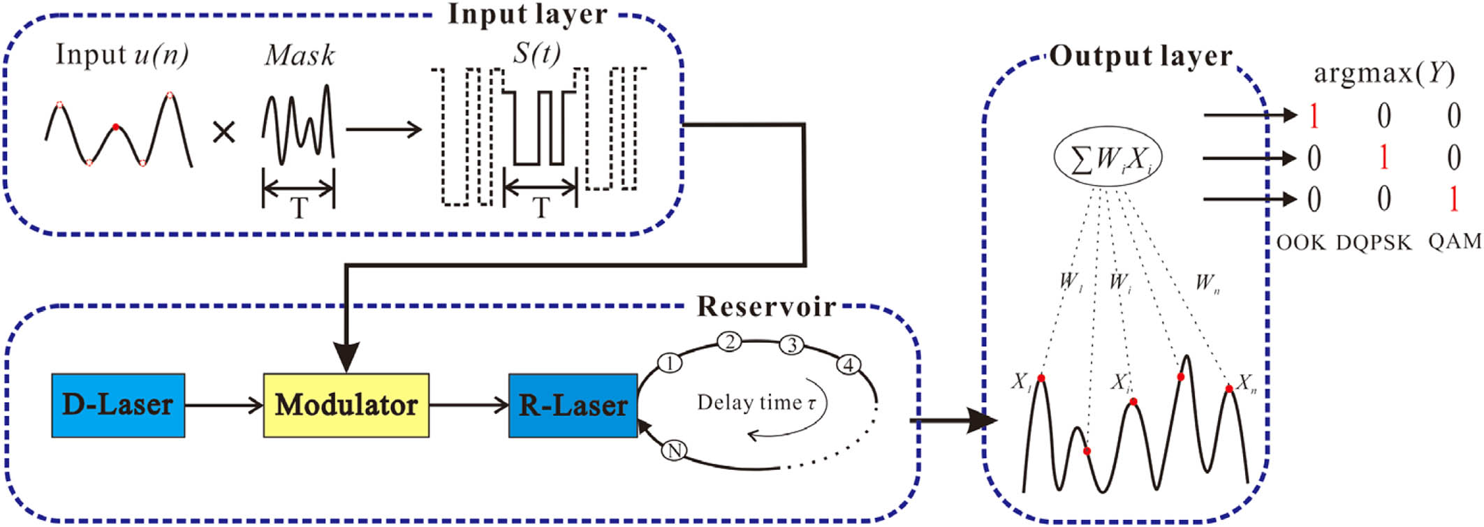
Figure 1 shows the schematic of the MFI based on the P-RC with semiconductor lasers. The whole system consists of three parts: input layer, reservoir, and output layer. In our implementation, the various modulation formats (OOK, DQPSK, QAM) commonly used in long-haul optical communication systems obtained their amplitude feature u(n) through asynchronous sampling. Specifically, the input u[n] is generated in the following way: 10 Gbps OOK, 40 Gbps DQPSK, and 100 Gbps 16QAM signals transmit over the emulated communication channel with different optical signal-to-noise ratios (OSNRs)/chromatic dispersions (CDs)/differential group delays (DGDs) and are then asynchronously sampled at a sampling rate of 500 MSa/s in a duration time of 0.2 ms to obtain 100,000 amplitude samples. After normalizing all of the sampled amplitudes, we form the associated asynchronous amplitude histograms (AAHs) containing 100 bins as shown in the following Fig. 3. Finally, 11,700 sample data sets are generated and used as the input information u[n]. The input information is a one-dimensional data vector u(n), where n∈Z is the discrete time. In the input layer, u[n] is preprocessed and multiplied by a mask sequence, which plays the role of random weight connections from the input to the reservoir layer. Note that different kinds of mask sequences can induce different effects on the RC performance. In the simulation, we actually investigated three kinds of commonly used mask signals, which are binary [38], six-level [39], and chaos masks [40], respectively. After analyzing their effect on the identification performance in the following Section 3, we finally select the chaos signal as the mask for RC. The amplitude feature u(n) first undergoes a sample-hold operation, where each sampling point has a duration of T and then is multiplied by a chaos mask sequence with a length of T. The resulting sequence S(t)=Mask×u(n) is further injected into the following photonic reservoir.

In the reservoir, the optical signal from the drive laser (D-Laser) is modulated by the loaded signal S(t) from the input layer and then injected into the response laser (R-Laser) with a time-delayed optical feedback. Following ideas introduced in RC with the delay system, the input information generates nonlinear transient states in the context of previous input responses. This is because the induced transient states at time t depend on the output of the nonlinear node within the time interval [t−τ,t], with τ being the delay time. In addition, the dynamics of the delay system exhibit the properties of high dimensionality and short-term memory, which accord well with the requirements of the P-RC. Within one delay interval of length τ, the feedback delay loop contains N virtual nodes at each interval time θ (θ=τ/N). We denote these N equidistant points as “virtual nodes,” as their roles are actually analogous to the nodes of a traditional reservoir. The values of the delayed variable at each of the N points define the states of the virtual nodes, which show the transient response of the reservoir when the input information is at the specific time. The whole working process in the reservoir can be modeled by Eqs. (1) and (2) [30,40,41]: $$\begin{gathered} dE(t)dt=1+iα2{g[N(t)−N0]1+ε|E(t)|2−1τp}E(t)+kfτinE(t−τ)exp(−i2πντ) \\ +kinjτinEinj(t)exp(i2πΔνt)+2βN(t)χ(t), \end{gathered}$$(1)dN(t)dt=J−N(t)τs−g[N(t)−N0]1+ε|E(t)|2|E(t)|2,(2)where E is the slowly varying complex electric field and N is the average carrier density. The parameters kf and kinj represent the feedback strength of external cavity of the R-Laser and the injection strength from the D-Laser to the R-Laser, respectively. ν denotes the frequency of the free-running R-Laser, and Δν denotes the frequency detuning from the D-laser to the R-laser. J is the injection current. The carrier density at transparency N0=4.55×1023m−3, the linewidth-enhancement factor α=5.0, the differential gain coefficient g=1.414×10−12m3⋅s−1, the gain saturation coefficient ε=2.0×10−23, the internal cavity round-trip time τin=7.38ps, the photon lifetime τp=1.17ps, and the carrier lifetime τs=2.5ns, respectively. The feedback delay time τ is 8 ns, and duration T=τ·χ(t) is a white Gaussian noise with zero mean and unity variance, used to model the spontaneous emission noise. β is the strength of the spontaneous emission noise. [Note that the following simulation results are obtained at β=0, except for the results in Table 3, where β=1.5×10−6.] Considering that the input signal is multiplied with the mask being used to modulate the optical signal through phase modulation, the injected slowly varying complex electric field Einj is written as Eq. (3): Einj(t)=Idexp[iπS(t)],(3)where Id is the photon number of continuous-wave output from the D-Laser, Id=3.757×1020. S(t) represents the masked input signal.

In the output layer, the transient states of the R-Laser Xi are read out for training the connection weights Wi between the reservoir and the output layer as defined in Eq. (4). Specifically, the optimal readout weights are calculated using the ridge regression algorithm in our work. The final output target Y(n) of three identified modulation formats is provided by using one-hot encoding [42] as follows. In the training stage of the P-RC, each input vector u(n) has a corresponding M×1 binary vector Y with only one nonzero element. The location of ‘1’ in Y indicates the signal modulation format type: Y(n)=∑XiWi.(4)Once the training process of the P-RC is completed, we employ the error rate (ER) to evaluate the MFI performance by a separate set of data called testing data set as defined in Eq. (5). In the testing stage, the location of the largest element in each corresponding output vector v, argmax{v}, is used as an identifier of the signal modulation format. The identified modulation formats are compared with true ones, which are provided by labels Y of the testing data set. Herein, Q represents the total of the samples of the testing data set, while b is the number of erroneous identification samples: ER=bQ×100%.(5)

As mentioned before, we choose 10 Gbps OOK, 40 Gbps DQPSK, and 100 Gbps 16QAM modulation format signals commonly used in long-haul fiber communication systems to validate the feasibility of our MFI proposal based on the P-RC in simulations. As shown in Fig. 2, these signals with three modulation formats transmit over a 30 km standard single-mode fiber (SMF; dispersion coefficient is 16 ps/(nm · km), attenuation factor is 0.2 dB/km, and nonlinear coefficient is 1.27km−1·W−1), respectively. An erbium-doped fiber amplifier (EDFA) is used to add amplified spontaneous emission (ASE) noise into the signals, while a variable optical attenuator (VOA) is used to adjust the OSNRs. A CD and a polarization mode dispersion (PMD) emulator are used to introduce variable amounts of CDs and DGDs into the signal, respectively. After removing the redundant noise by an optical band-pass filter (BPF) and direct detection by a photodetector (PD), the resulting electrical signal is asynchronously sampled to form asynchronous amplitude histograms (AAHs). The OSNR ranges considered in this work are the ones used in practice for reliable data transmission with the abovementioned signal types. There are various losses in the signal transmission process of optical fiber. Specifically, we investigate the three types of signals in the following scenarios: (i) their OSNRs are adjusted, ranging from 12 to 26 dB through a VOA at a step of 1 dB; (ii) their CDs are set, ranging from −500 to 500 ps/nm via a CD emulator at a step of 80 ps/nm; (iii) their DGDs are located by a PMD emulator in the range of 0−20ps with a step of 5 ps. Here we want to point out that using a fixed length of standard SMF with different OSNR and CD following is a common method to simulate the transmission system for asynchronous amplitude histogram generation [11,43]. In this way, the OSNR and CD can be easily adjusted to obtain associated data. Thus, we also apply this method in our simulation. Note that the nonlinear effects are very weak in the 30 km fiber propagation, and thus their impact is almost negligible.

Based on the above scenarios, 11,700 samples of modulation format signals in total are collected, and the randomly selected subsets of this large data set are then used for training and testing the performance of the P-RC. The examples of amplitude histograms for OOK, DQPSK, and 16QAM signals after asynchronous sampling are typically shown in Fig. 3. Herein, the OSNRs in each column are 12, 19, and 26 dB from left to right, but the corresponding CD and the DGD are fixed at 80 ps/nm and 5 ps, respectively. From each column, it can be clearly seen that different modulation formats exhibit distinct shapes. Even though the associated shapes change with various OSNRs from the first column to the third column, three types of modulation formats maintain distinct characteristics for each format. Therefore, the characteristic features of the asynchronous amplitude histograms have been widely accepted to be exploited for MFI.

In the following, we will use the features from the asynchronous amplitude histograms to train and test the P-RC so that MFI can be realized. At the first stage, we confirm the appropriate number of samples and the optimized size of the virtual nodes in the P-RC for high efficiency. In our scheme, we adopt the commonly used k-fold cross-validation algorithm [44] to eliminate the impact of the specific division of the available data samples between training and testing. This means that the entire process of training and testing is repeated k times (with k=5) on the same data, but each time with a different assignment of data samples to each of the two stages. The final ER in testing on the y axis is the mean across these k=5 runs. We compared the identification results with different types of mask signals (the binary mask, six-level mask, and chaos mask) by varying the sample numbers. The binary mask consists of a piecewise constant function with a randomly modulated binary sequence {−1, 1}. Similar to the binary mask, the six-level mask is composed of a random sequence {±1, ±0.6, ±0.3}. The chaos mask signal is generated from another semiconductor laser with optical feedback [45]. Here the amplitude of the chaos mask is rescaled so that the standard deviation of the chaos mask is set to 1 and the mean value is set to 0. As shown in Fig. 4(a), the ER tends to be a stationary value when the sample number reaches around 2700. Meanwhile, it is clear that the chaos mask performs better than the other two types of masks. Thus, we select the chaos signal as the final mask in the following simulation. On the other hand, it can be observed that no matter whether the number of virtual nodes N in the P-RC is set as 300 or 400, the ER exhibits the same changing trend. Meanwhile, it should be noted that the ER corresponding to the virtual node number N=400 is lower than that in the other cases of N=300.

As shown in Fig. 4(b), the ER decreases with the increase of the sample number and tends to be a stationary value. The red curve is the corresponding red curve (chaos mask) in Fig. 4(a). Consequently, 2700 samples of modulation signals and the virtual node number N=400 are selected in our simulation.

Furthermore, we analyze the effect of the four key parameters in the P-RC layer on the MFI performance, which are the injection strength kinj from the D-laser to R-laser, feedback strength kf of the R-laser, bias current IR of the R-laser, and frequency detuning Δν from the D-laser to R-laser. Figure 5 depicts the associated influence of the injection strength. When there is no input, the P-RC is a typical master-slave laser configuration. From its bifurcation diagram [Fig. 5(a)], one can observe that when the injection strength kinj is less than 0.21, the output of the P-RC layer is in a chaotic state. With increase of the injection strength kinj, the P-RC laser changes from the periodic oscillation state to a single-cycle state. On the other hand, Fig. 5(b) shows the dependence of the identification ER on the injection strength when the input is considered. It can be seen from Fig. 5(b) that the ER is first decreased but then increased with the increase of the injection strength kinj. The lowest ER of 5.21% can be obtained when the optimum value of injection strength kinj is equal to 0.2. Comparing its corresponding bifurcation diagram [Fig. 4(a)], it can be found that when kinj is around 0.2, the delay-coupled semiconductor laser reservoir system in the absence of input works at the edge of the chaos region. This phenomenon is consistent with that in Ref. [15], where electrical reservoir computing based on a single dynamical node is used for standard benchmarking tasks such as spoken digit recognition and nonlinear time series prediction.

Figure 6 shows the effect of the feedback strength kf of the R-laser on the identification performance. Here the injection strength kinj is set at 0.2, while other parameters remain unchanged (IR=1.3Ith and Δν=−10GHz). When the feedback strength kf varies from 0.01 to 0.35, it can be seen from the corresponding bifurcation diagram in Fig. 6(a) that the output of the reservoir without the input follows a quasiperiodic route to chaos with the increase of the feedback strength kf. After the input is considered, the final identification ER of our P-RC in Fig. 6(b) is decreased at first and then increased with increasing feedback strength kf. When the feedback strength kf is 0.15, the ER reaches a minimum value of 5.09%. When the feedback strength grows, the system is in the chaotic state and is more sensitive to changes in initial conditions. So the identification performance will decline.

Figure 7 illustrates the influence of the bias current IR of the R-laser in the system. In the analysis, the injection strength kinj and the feedback strength kf are set to be 0.2 and 0.15, respectively. Figure 7(a) is the corresponding bifurcation diagram of the output optical intensity versus the bias current IR of R-Laser. As can be seen, the RC subsystem will gradually leave a single-cycle state to the chaotic region when the bias current of the R-Laser increases from 1.01Ith to 1.6Ith. Note that Ith corresponds to the threshold current of the R-Laser. On the other hand, the identification ER in Fig. 7(b) first decreases and then increases with the increase of IR. Finally, a minimum ER of 4.25% can be obtained when the bias current of the R-Laser equals 1.25Ith.

Figure 8 investigates the influence of the frequency detuning Δν between the D-Laser and the R-Laser on the identification results. Figure 8(a) gives the bifurcation diagram as a function of the frequency detuning Δν. In the bifurcation diagram, the RC without the input can be observed in a single-cycle state when the frequency detuning Δν is −15GHz. With the increase of the frequency detuning Δν, it starts to enter a chaotic state at Δν=−10GHz. Figure 8(b) shows that the identification ER exhibits the same changing trend as Figs. 5(b), 6(b), and 7(b). That is, the ER decreases first and then increases with the increase of frequency detuning Δν. When the frequency detuning Δν is −10GHz, the ER can be reduced to a lowest value of 4.07%. Obviously, this best identification result is obtained at the edge of the chaos region by contrast with the bifurcation diagram. In this state, the RC has an infinite dimensional space so the input signal is mapped to the higher dimensional space and achieves the optimal identification results.

After the above processes, all key parameters in our P-RC can be adjusted to reach the optimum state as follows. (i) The number of virtual nodes N is chosen to be 400. (ii) The injection strength kinj from the D-laser to the R-laser is set to be 0.2. (iii) The feedback strength kf of the R-laser is set as 0.15. (iv) The bias current IR of the R-Laser is 1.25Ith. (v) The frequency detuning Δν between the D-Laser and R-Laser is set to −10GHz.

Under these conditions, we utilize the P-RC system to identify 1000 test cases with each type of modulation format for a considerable range of OSNRs (12-26dB), CDs (−500-500ps/nm), and DGDs (0-20ps). Table 1 lists the associated test results of the proposed MFI technique through combining the ridge regression algorithm with the laser-based P-RC system. From it, one can confirm that the identification accuracies of OOK, DQPSK, and 16QAM signals can reach 95.1%, 95.7%, and 95.5%, respectively. These simulation results demonstrate that the proposed technique can effectively classify the modulation formats in fiber communication with an overall estimation accuracy of more than 95% and also in the presence of various link impairments such as OSNR, CD, and DGD. Meanwhile, in order to check the performance of our proposal, we also analyzed the MFI accuracy using only the ridge regression algorithm. In this case, the whole system only contains two layers: the input and output layers. The whole training process is as follows. The resulting sequence S from the input layer and the target matrix Y are directly used to calculate the final output connection weight W by means of the ridge regression algorithm. That is, there is no nonlinear mapping induced by the reservoir layer. The associated results on identification accuracies for different modulation formats are shown in Table 2. It is evident that the identification accuracies of all three modulation formats in the system only using the ridge regression algorithm are less than 76%. Therefore, we confirm that the identification accuracies can be significantly improved based on the proposed P-RC MFI system in our work.

Further, we investigate the influence of spontaneous emission noise on the performance of the P-RC. Table 3 shows the identification accuracies for different modulation formats using the MFI technique through the P-RC system under a typical spontaneous emission β=1.5×10−6 [46]. Comparing Table 1 and Table 3, one can find that our P-RC is extremely robust against spontaneous emission noise. That can be explained by the fact that the modulation format identification is a classification task that only requires a winner-takes-all decision. Note that the noise from the photodetector is additive, which can be eliminated using balance detection technology. Thus, the detection noise is not considered in this work.

Finally, we want to point out that direct comparison with other works is difficult in modulation format identification as mentioned in Refs. [12,47]. There are two main reasons for this difficulty. (i) There is no single unified database available. When different modulation formats with different symbol rates are applied, different accuracies will result for NN-based modulation format identification. (ii) Identification accuracy is frequently reported as a function of OSNR and CD. There are no benchmarking systems universally agreed upon these indexes. For instance, Guesmi et al. reported an identification accuracy of 90% for 16 Gbps QPSK and 16QAM when the OSNR is 14−26dB and the CD is 800 ps/nm [48]. Saif et al. showed an identification accuracy of 98% for 10 Gbps QPSK and 16QAM when OSNR is about 20 dB; however, when the symbol rate is enhanced into 20 Gbps, the associated identification accuracy is decreased to 90% [49]. Xiang et al. reported an identification accuracy of 100% for 28 Gbps QPSK and 16QAM when the CD is −60−60ps/nm; but when the CD is in the other range, the identification accuracy is decreased below 90% [43].

There are at least two benefits to the P-RC. (i) High speed. Our P-RC is based on the all-optical nonlinearity of laser diodes. Such a system might even reach processing speeds at the level of 100 GHz using off-the-shelf photonic components for telecommunication applications [50]. (ii) Low energy consumption. At this stage we can only provide a conservative estimate, according to Ref. [16]. Our all-optical transient computing scheme, including all-optical data input and readout hardware, would be of the order of 10 mJ per signal, compared with 2 J per signal required by a standard desktop computer.

In addition, the current accuracy level in this work is mainly constricted by the number of used nodes due to the limited sample size. Once the sample size is sufficiently large (that means more nodes are fully trained), there are two approaches to further achieve higher accuracy levels with P-RC. One is to improve the complexity of the mask [40]. In P-RC, the mask is equivalent to the input connection weight in the traditional RC. It can bring rich nonlinear states for P-RC and thus map the input data into a high-dimensional space. So it is expected that using a more complicated random signal (such as amplified spontaneous noise) as the mask may further enhance the identification accuracy. The other is to introduce the multiple feedback loops [30]. Usually, the P-RC system with multiple optical feedback results in a much more complex response of the R-laser compared to that with a single optical feedback. Consequently, higher dimensional transformation of the input signal and thus higher accuracy levels may be achieved with P-RC.

In this paper, we propose a simple MFI technique for fiber-optic communications by using P-RC trained with amplitude features extracted from the OOK, DQPSK, and 16QAM signals through asynchronous sampling. Numerical results demonstrate over 95% identification accuracy for three widely used modulation formats in various situations under OSNRs (12−26dB), CDs (−500−500ps/nm), and DGDs (0−20ps). Considering the good performance and its conceptual simplicity, it can be expected that P-RC may provide an efficient tool for realizing the wide application of MFI in future fiber communication systems.