
Junyan Li, Na Qian, Shiyu Hua, Weiwen Zou. Optimization of optical signal-to-distortion ratio in a channel-interleaved photonic ADC via a coherent multi-frequency RF driver[J]. Chinese Optics Letters, 2021, 19(8): 083901
- Chinese Optics Letters
- Vol. 19, Issue 8, 083901 (2021)
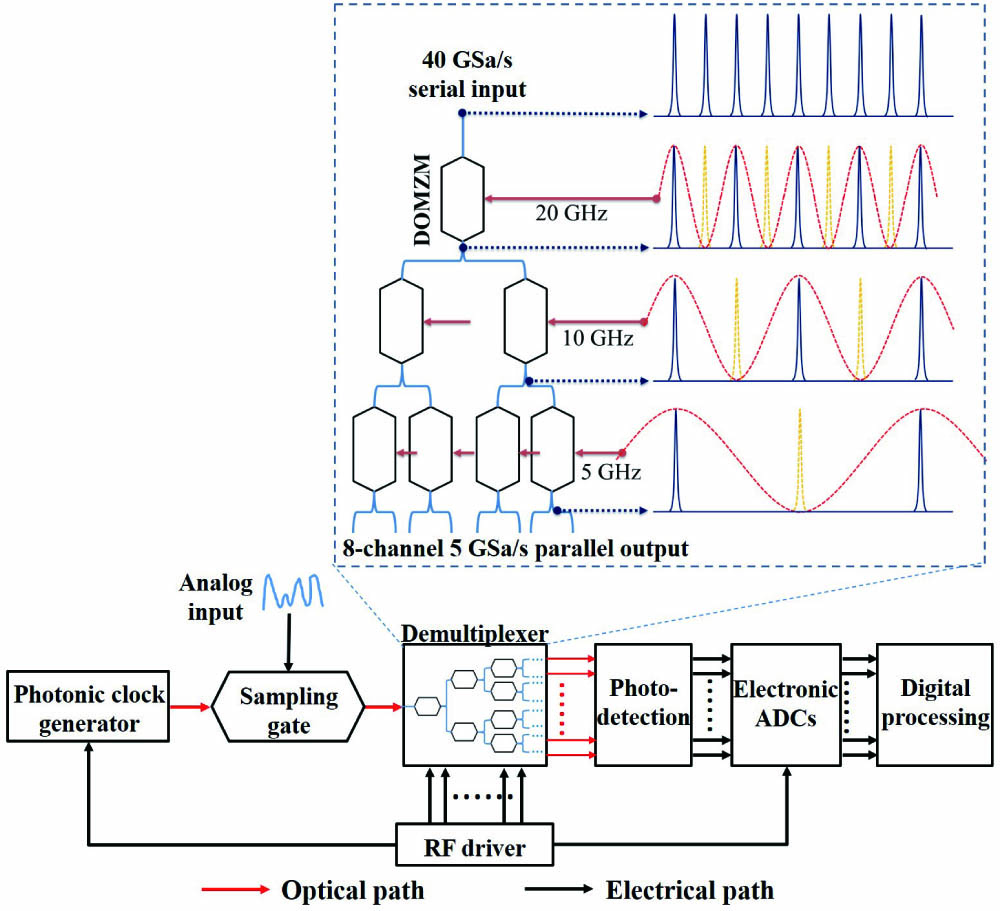
Fig. 1. Schematic of a 40 GSa/s eight-channel PADC with a channel-interleaved demultiplexer based on a binary tree of dual-output Mach–Zehnder modulators (DOMZMs). The inset shows the working mechanism of a three-class demultiplexer, which converts sampling series of 40 GSa/s into eight parallel channels of 5 GSa/s.
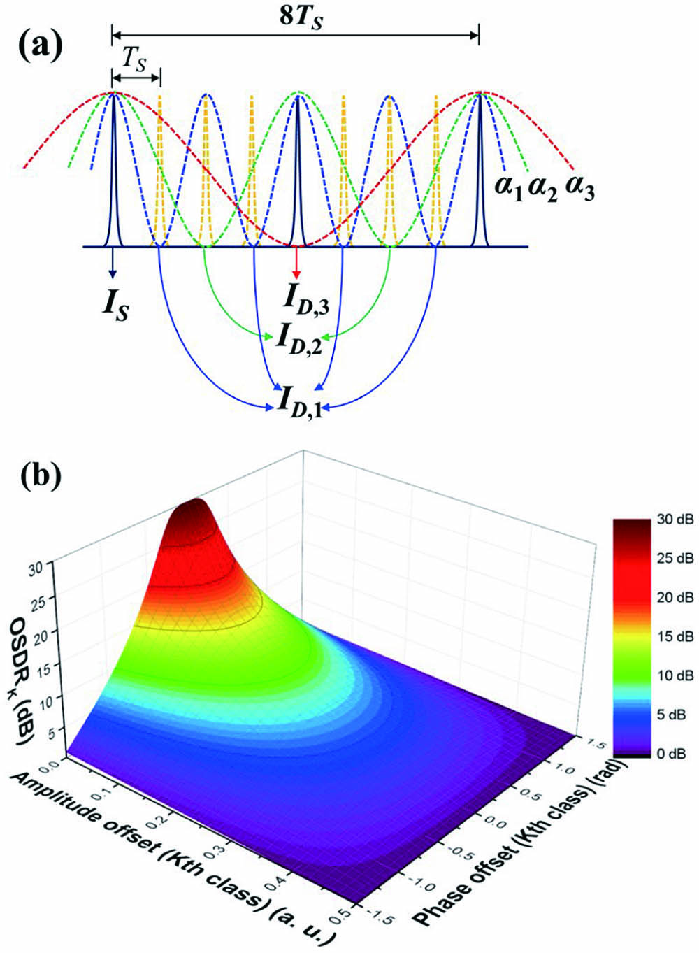
Fig. 2. (a) Schematic of the selected pulse and induced distortions in a three-class DOMZM-based demultiplexer. αK is the switching response of one DOMZM in the Kth class (K = 1, 2, 3), IS is the intensity of the selected pulse, and ID,K is the intensity of the distortions induced in the Kth class. (b) Simulated optical signal-to-distortion ratio (OSDR) at each single-class DOMZM versus both amplitude and phase offsets of the RF driver signal. The colors on the surface refer to the magnitude of the OSDRK. The subscript K represents an integer, which can be 1, 2, or 3.
Fig. 3. (a) Design schematic of the microwave-chip-based RF driver and (b) its photo. PS, power splitter; LNA, low noise amplifier; PA, power amplifier; FM, frequency multiplier; FD, frequency divider; VA, variable RF attenuator; VPS, variable RF phase shifter; BPF, band-pass filter; EADC, electronic ADC.
Fig. 4. (a)–(d) Typical frequency responses of the output ports of the RF driver module with different frequencies and different power. The adjustment precision in power is 0.5 dB and 6 bits. The working frequencies and power are marked as black dots. (e)–(h) The spectra of the output driver signal from the ports in (a)–(d). All plots are marked with the frequency and the power.
Fig. 5. Temporal waveforms of demultiplexed series from each class under different conditions of the amplitude and phase of RF driver signals in (a)–(c) first class, (d)–(f) second class, and (g)–(i) third class. (j) Comparison between the theoretically estimated and the experimentally measured OSDRK according to (a)–(i). The measured values are labeled, and the contours are based on the theoretical model.
Fig. 6. Temporal waveforms of final demultiplexed 5 GSa/s series under the conditions depicted in Figs. 5(a) –5(i) in each class: (a) Fig. 5(a) as the first class, Fig. 5(d) as the second class, and Fig. 5(g) as the third class; (b) Fig. 5(b) as the first class, Fig. 5(e) as the second class, and Fig. 5(h) as the third class; (c) Fig. 5(c) as the first class, Fig. 5(f) as the second class, and Fig. 5(i) as the third class. The OSDRK in each class is labeled as depicted in Fig. 5(j) . The final OSDR is measured and compared with its theoretical estimation, which increases along with the OSDRK in each class.

Set citation alerts for the article
Please enter your email address
© Copyright 2018-2021 | Chinese Laser Press. All Rights Reserved 沪ICP备15018463号-20