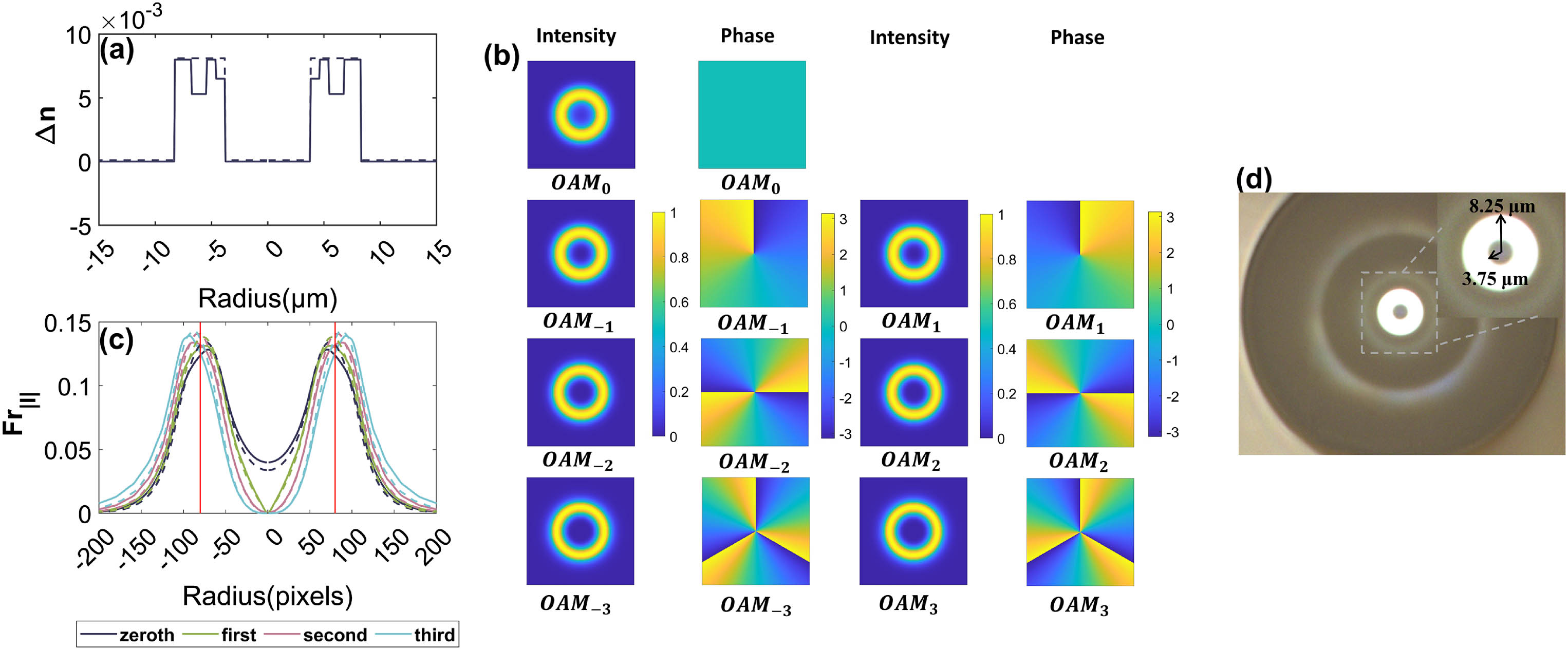
Fig. 1. Refractive index distribution and mode characteristics of the RCF used for demonstration. (a) Refractive index profile of the RCF. (b) The intensity distribution and phase distribution of each OAM mode. (c) The radial field functions of OAM modes with different azimuthal orders. The actual length range is consistent with (a). (d) The cross-section image of the RCF captured by a microscope.

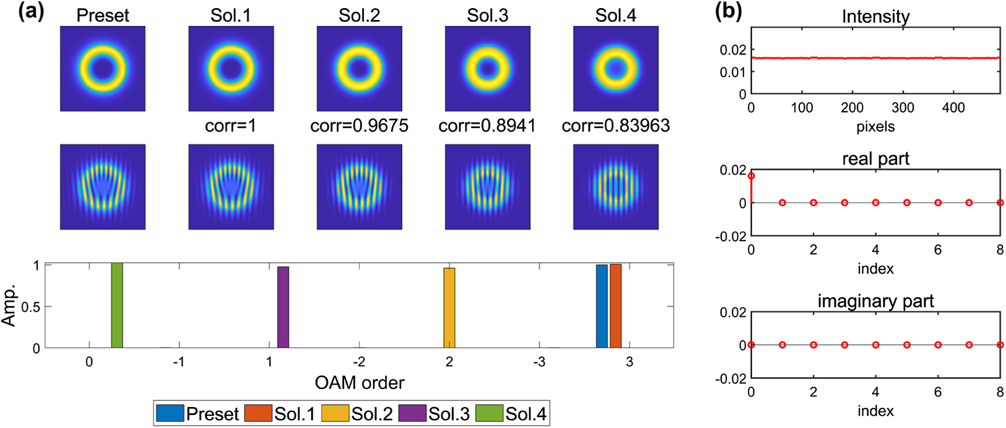
Fig. 2. Demonstration for solving the equation group in the pure-mode situation. (a) Intensity patterns, interference patterns, and amplitude spectrum of the preset pure third-order OAM mode and four analytic solutions of Eq. (4). (b) The intensity of the azimuthal sampling sequence, the real part and imaginary part of its Fourier spectrum.

Fig. 3. Demonstration for solving the equation group in the impure-mode situation. (a) Intensity patterns, interference patterns, and amplitude spectrum of the preset pure third-order OAM mode and four numerical solutions of Eq. (4). (b) The intensity of the azimuthal sampling sequence, the real part and imaginary part of its Fourier spectrum.

Fig. 4. Different simulation results of purity measurement for impure modes. (a1)–(a3) Intensity patterns, interference patterns, preset and recovered amplitude spectra. (b1)–(b3) Intensity patterns, preset and recovered amplitude spectra, and the corresponding initial value of iteration.

Fig. 5. Accuracy corresponding to mode purity when the fiber supports different numbers of modes. The highest azimuthal order of modes in (a)–(e) is from 3 to 7.

Fig. 6. Accuracy corresponding to the noise level and the size of input images. (a) The accuracy corresponding to the noise level. (b) The accuracy corresponding to the size of input images.

Fig. 7. Similarity of the radial field functions when fiber parameters change. The color of each cell represents the value of ΔFr when the fiber parameter is located in the lower left cell line. (a) Δn=0.010, (b) Δn=0.015, (c) Δn=0.020, and (d) Δn=0.030.

Fig. 8. Schematic diagram of the polarization test method.

Fig. 9. Experimental setup. (a) Algorithm verification device. (b) Mode purity testing device. SMF, single-mode fiber; OC, optical coupler; PC, polarization controller; SLM, spatial light modulator; QWP, quarter-wave plate; RCF, ring core fiber; Pol., polarizer; OL, objective; NPBS, unpolarized beam splitter.

Fig. 10. Schematic diagram of the process of the proposed purity measurement method. (a) Flow chart of the proposed purity measurement method. (b) Determination of the optical axis in the camera. (c) The cropped image. The red circle represents the sampling radius. (d) The intensity of the azimuthal sampling sequence, the real part and imaginary part of its Fourier spectrum. (e) Recovered amplitude spectrum.

Fig. 11. Demonstration of how different experimental factors affect the algorithm’s precision. (a) Preset images, reconstructed images, and their correlations under different conditions. (b) Recovered amplitude spectrum under different conditions. (c) Recovered phase spectrum under different conditions.

Fig. 12. Experimental results of the optical field which appears as a single near-pure OAM mode at different polarizations. (a1)–(a3) The captured images, reconstructed images, measured amplitude spectrum, and the mode purity (P). (b1)–(b3) The captured images, reconstructed images, measured amplitude spectrum, predicted amplitude spectrum, the mode purity (P), and the error of amplitudes (ϵA).

Fig. 13. Experimental results of the optical field which appears as the superposition of two fourth-order OAM modes at different polarizations. (a1)–(a3) The captured images, reconstructed images, measured amplitude spectrum, and the mode purity (P). (b1)–(b3) The captured images, reconstructed images, measured amplitude spectrum, predicted amplitude spectrum, the mode purity (P), and the error of amplitudes (ϵA).

Table 1. Comparison with the State-of-the-Art Methods^a