• Photonics Research
  • Vol. 11, Issue 9, 1592 (2023)
Zekun Shi, Baiwei Mao, Zhi Wang, and Yan-ge Liu*
Author Affiliations
  • Institute of Modern Optics, Tianjin Key Laboratory of Micro-scale Optical Information Science and Technology, Nankai University, Tianjin 300350, China
  • show less
    DOI: 10.1364/PRJ.494864 Cite this Article Set citation alerts
    Zekun Shi, Baiwei Mao, Zhi Wang, Yan-ge Liu. Accurate mode purity measurement of ring core fibers with large mode numbers from the intensity distribution only[J]. Photonics Research, 2023, 11(9): 1592 Copy Citation Text show less

    Abstract

    Mode purity measurement is crucial for various applications utilizing few-mode fibers and related devices. In this paper, we propose a simple and accurate method for measuring the mode purity of the output optical field in few-mode ring-core fibers (RCFs). Mode purity can be calculated solely from the outgoing intensity distribution with high precision. This method is theoretically capable of measuring the mode purity of RCFs that support orbital angular momentum modes with an infinite number of azimuthal orders and has strong applicability to various RCF types and image qualities simultaneously. We demonstrate our approach numerically and verify it experimentally in a few-mode RCF supporting four (five) mode groups at 1550 (1310) nm. A polarization test method is proposed to verify its accuracy. We believe that this straightforward and cost-effective characterization method for RCFs and RCF-based devices can promote the development of mode-division multiplexing technology and its applications.

    1. INTRODUCTION

    Orbital angular momentum (OAM) beams are characterized by a spiral wavefront and are widely used in high-capacity communication [13], optical metrology [4], optical tweezers [5,6], and data storage [7,8]. As cylindrical waveguides, few-mode fibers (FMFs) serve as a natural container for OAM modes. In an ideal OAM fiber, each OAM mode is orthogonal and able to carry independent information [911], which significantly increases the communication channel capacity or the degrees of freedom for multi-parameter sensing applications. However, the severe unpredictability of inter-mode coupling in actual fibers poses a significant challenge, hindering the reliability of using each OAM mode as a controllable unit and limiting the application of FMFs in various fields. Compared to conventional FMFs, few-mode ring core fibers (RCFs) are better suited for the stable propagation of OAM modes due to its ring-shaped mode field distribution [2,12,13]. RCFs have also been demonstrated to achieve weak coupling between higher-order modes (HOMs) and reduce the emergence of radial HOMs [14,15]. These advantages increase the capacity of OAM multiplexing communication systems and reduce the complexity of signal processing.

    In communication and other applications based on RCFs, it is crucial to design FMFs with lower cross talk as well as to design devices with more efficient mode conversion and multiplexing capabilities [14]. This stimulates the demand for performance characterization of these FMFs and devices, one key issue being the purity measurement of the spatial modes actually transmitted in the fiber. For optical fibers, high-precision purity measurement methods mean accurate characterization of inter-mode cross talk [15,16], which can reflect the feasibility of fiber design methods and may reveal more details about the physical mechanism of inter-mode coupling, thereby pointing to paths for further suppression of inter-mode coupling. For OAM spatial [1719] and all-fiber [2022] devices, experimental measurements of optical field purity can provide guidance for device development and evaluate device performance in application, as pure mode sources are important for reducing system complexity. In addition to characterizing the performance of fibers and fiber devices, simple purity measurement methods can also provide new ideas for compensating for inter-mode coupling, to solve the dilemma of FMFs in different fields, especially when combined with fiber transmission matrix measurement and inversion [23,24].

    In principle, measuring mode purity requires determining not only the major mode component in FMFs or FMF-based devices but also all possible other mode components. Traditionally, researchers determine the main component of an unknown optical field by examining the shape of the mode pattern or interferogram [25,26]. In the mode pattern, modes with different azimuthal orders exhibit varying numbers of lobes. In the interferogram, they exhibit different spiral or fork wire patterns. However, if the mode is not pure, the mode pattern and interferogram are complex, and determining each mode component to calculate the purity of the main component remains challenging. This problem is often referred to as the measurement of OAM spectrum or mode decomposition. To solve this problem, various methods based on diffraction, coordinate transformation, and interference have been proposed [18,19,23,2735]. However, when applied to the measurement of mode purity of RCF-based devices, these methods face some challenges.

    The methods based on diffraction [18,27] and coordinate transformation [19,28,29] principle usually require a spatial light modulator (SLM) and complex experimental configuration and cannot be simply adapted to the purity measurement of HOMs in ring core fibers. The fundamental mode in ring core fibers is doughnut shaped in the near-field condition, and has quite different mode characteristics from the intrinsic fundamental mode in free space, which further increases the complexity of the actual configuration. Since most mode converters use the fundamental mode as the source, it is usually a non-negligible impurity that should be measured simply and accurately.

    The methods based on the interference principle can be divided into three categories. The first category utilizes the different propagation constants of different modes, such as the spatially and spectrally resolved imaging method [30], swept-wavelength interferometry measurement [16], and vector network analyzer (VNA) measurement [36]. These methods are general and useful for characterizing fibers with an unknown structure, but their application is limited by the requirement for expensive tunable lasers or VNAs. Additionally, these methods require long optical fibers to generate sufficient group delay between different modes and cannot distinguish degenerate OAM modes with similar propagation constants. The second category takes advantage of the principle that different mode combinations result in different intensity distributions at the fiber output [23,3133,37]. These methods do not require complex equipment and can directly measure the mode components using numerical algorithms, indicating strong applicability. However, the number of modes that can be resolved by these methods is limited due to their sensitivity to noise and initial value of iteration or dependency on long-term neural network training. As a result, it is challenging to apply them to purity measurements in RCFs with a large number of modes. In previous experimental reports, the highest azimuthal order of the modes supported by FMFs is only 3 [23]. The third category requires a reference beam to obtain the phase distribution of the output optical field and calculates all mode components using the mode orthonormal property [34,35,38]. These methods require accurate alignment of the optical path and interference stability for in situ measurement. However, in practical applications of FMFs, achieving phase stability can sometimes be difficult to attain.

    In this study, we propose a straightforward and precise technique to measure the mode purity of the output optical field in RCFs. We establish an equation that links the intensity distribution to the mode components. Once the main component of the optical field is known, the amplitude of each degenerate mode can be obtained by measuring the output intensity distribution once, enabling the calculation of mode purity. To verify the accuracy and effectiveness of this technique, we propose a simple polarization test method that uses only a polarizer to verify if each component is correctly recovered at once. We demonstrate our approach numerically and verify it experimentally in a few-mode RCF supporting four (five) mode groups (MGs) at 1550 (1310) nm. All simulation and experimental results confirm the applicability and accuracy of our method. The proposed method has the advantages of simple equipment, easy implementation, high accuracy, and noise resistance. Most importantly, the performance of this method will hardly decrease as the number of fiber modes increases, so theoretically it can be used to measure the purity of RCFs that support OAM modes with an infinite number of azimuthal orders.

    To better highlight the advantages and innovations of the proposed technology, we compare it with several state-of-the-art techniques based on similar principles, specifically, the second and third categories of methods based on the interference principle. The comparison is shown in Table 1. The phase measurement methods allow for the analysis of a sufficient number of modes for the ring core fibers, but they require reference light, precise optical alignment, and interference stability, which is not conducive to on-site measurements in practical applications. In addition, for some complex active devices such as pulsed lasers [40,41], obtaining a reference beam would take more experimental effort. Compared to other intensity-only measurement methods, our approach only requires information about the main mode component. It does not need any neural network training but can achieve mode purity measurements of ring core fibers with large mode numbers in practical noise level. Therefore, the proposed technique can be a good candidate for characterizing and evaluating the performance of RCFs and RCF-based active and passive devices.

    Comparison with the State-of-the-Art Methodsa

    MethodReference BeamTrainingMain Component InformationLmax in SimulationLmax in ExperimentsSNR Requirement (Lmax=3)References
    Coaxial interferenceYNN8[35]
    Off-axis interferenceYNN >10[34,39]
    Neural networkNYN63[23]
    Matrix operationNNN82>33  dB[31,33]
    This paperNNY745  dB

    Lmax, the highest azimuthal order of modes; SNR, signal-to-noise ratio; Y, there is a requirement for the condition; N, there is no requirement for the condition.

    2. THEORY AND SIMULATION

    A. Principle of Purity Measurement

    To accurately measure the mode purity of the output optical field in RCFs, it is crucial to understand their mode field characteristics. In this study, we used a specific RCF that supports four MGs at a wavelength of 1550 nm as an example. This fiber was designed and fabricated to minimize inter-MG coupling and has been demonstrated to enable the implementation of OAM communication over a distance of 100 km [42,43]. The relative refractive index difference (Δn) of the fiber core is shown in Fig. 1(a). The fiber cladding diameter is 125 μm, and the ring core inner and outer radii are 3.75 μm and 8.25 μm, respectively. The ring core can also be seen in the cross-section image of the RCF captured by a microscope shown in Fig. 1(d). The maximum Δn in the refractive index profile (RIP) is equal to 0.008. In order to decrease micro-perturbation-induced inter-MG coupling, two notches are introduced in the RIP. For the first one from 3.75 to 4.6 μm, Δn=0.0065. For the second one from 5.4 to 6.8 μm, Δn=0.0053. Using the finite element method with commercial software COMSOL, we calculated the intensity and phase distribution of each OAM mode at 1550 nm, as depicted in Fig. 1(b). The four MGs have different azimuthal orders: zeroth order (OAM0), first order (OAM±1), second order (OAM±2), and third order (OAM±3). Each fiber mode in Fig. 1(b) further has two orthogonal polarization states (x- and y-polarized states). Additionally, modes within the same MG share the same intensity distribution and radial field function (RFF). Figure 1(c) shows the normalized RFFs Fr|l|(r) with different azimuthal orders.

    Refractive index distribution and mode characteristics of the RCF used for demonstration. (a) Refractive index profile of the RCF. (b) The intensity distribution and phase distribution of each OAM mode. (c) The radial field functions of OAM modes with different azimuthal orders. The actual length range is consistent with (a). (d) The cross-section image of the RCF captured by a microscope.

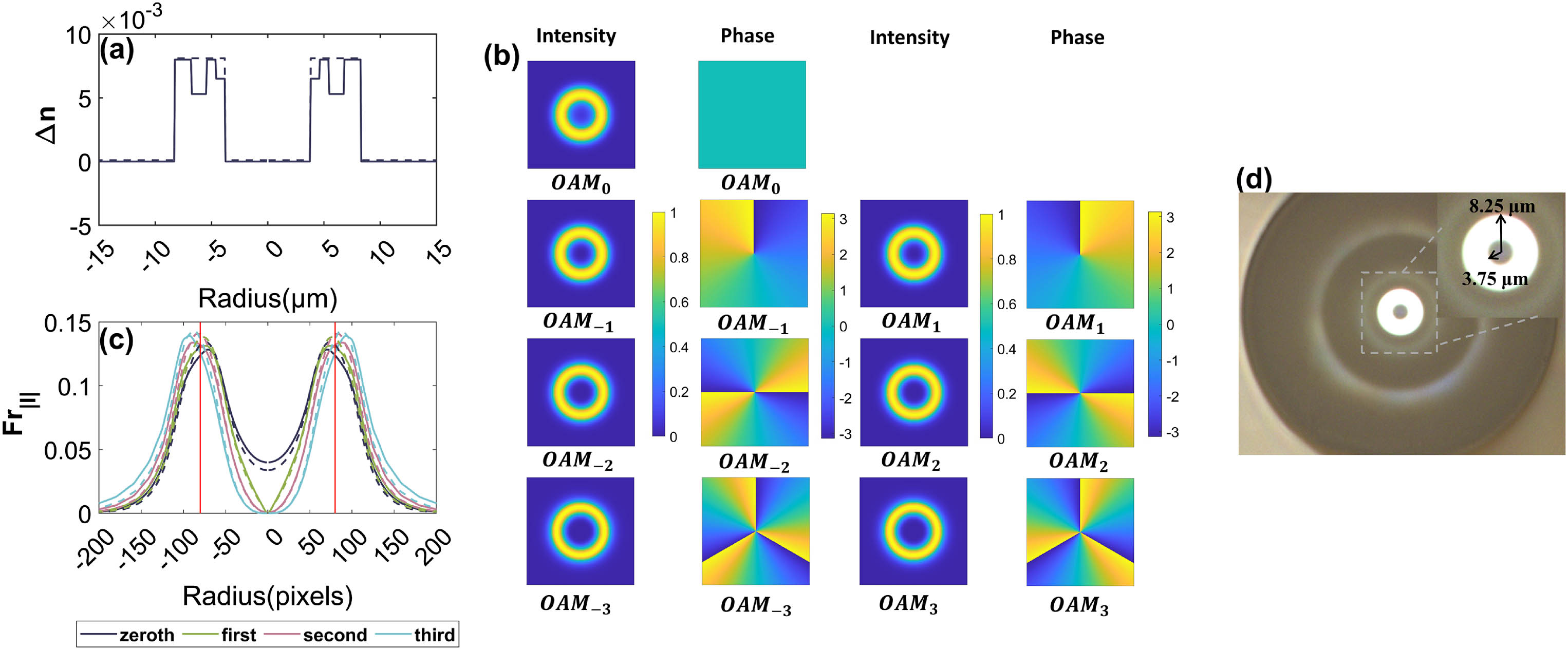
    Figure 1.Refractive index distribution and mode characteristics of the RCF used for demonstration. (a) Refractive index profile of the RCF. (b) The intensity distribution and phase distribution of each OAM mode. (c) The radial field functions of OAM modes with different azimuthal orders. The actual length range is consistent with (a). (d) The cross-section image of the RCF captured by a microscope.

    Compared to conventional FMFs, where the radial field distribution of modes is dominated by the Bessel function and Laguerre Gaussian function, the RCF exhibits a distinct feature in which each Fr|l|(r) is similar as shown in Fig. 1(c), indicating highly overlapping mode field distributions for each mode. Removing the two notches designed to decrease micro-perturbation-induced inter-MG coupling does not significantly alter the RFFs [dotted lines in Figs. 1(a) and 1(c)], suggesting that the radial field distribution is primarily caused by the high refractive index region in the RIP and is almost unaffected by other design factors. Although our simulation and experimental discussions focus on this particular fiber, our findings are applicable to all types of RCFs with similar RFFs.

    In the following, we will focus on one polarization state, for example the x-polarized state. However, the analysis can easily be extended to the full vector field by applying the same method to both orthogonal polarization components. The optical field in the fiber can be expressed as EL(r,θ)=l=LLρl·φl(r,θ)=l=LLAleiαl·Fr|l|(r)eilθ=l=LLCl(r)eiαleilθ,where Cl(r)=AlFr|l|(r), r and θ are the radius and azimuth coordinates, φl(r,θ) are the electric fields of OAM modes, l are the azimuthal orders (L is the highest order), ρl=Aleiαl are complex mode coefficients representing amplitudes and phases of the corresponding modes, and Fr|l| are the RFF of modes.

    It is worth noting that the OAM modes here are not only the specific modes in the fiber, but also one of the three mode bases in weak-guiding FMFs. The remaining two mode bases are linear polarization (LP) modes and cylindrical vector (CV) modes, respectively. These three mode bases are related by a complete transformation relationship [44,45], so that once the amplitudes and phases of each mode in the OAM mode base are fully characterized, the amplitudes and phases of each mode in the LP and CV mode bases can be obtained immediately via the transformation relationship, and vice versa.

    To measure the mode purity, we need to determine the amplitudes of each OAM mode from the intensity distribution of the outgoing light. In the near-field condition, the mathematical expression for the intensity distribution is given by Eq. (2): IL(r,θ)=|EL(r,θ)|2=Σl=LLCl2(r)+ΣΔl=12LΣl=L+ΔlL2Cl(r)ClΔl(r)cos[Δl·θ+(αlαlΔl)],where Δl=|l2l1|(Δl=1,2,,2L1,2L).

    If a certain radius r=r0 is chosen, IL(r,θ) is reduced to an azimuthal sampling one-dimensional sequence: IL(r0,θ)=Σl=LLCl2(r0)+ΣΔl=12L{[Σl=L+ΔlL2Cl(r0)ClΔl(r0)cos(αlαlΔl)]cos(Δl·θ)[Σl=L+ΔlL2Cl(r0)ClΔl(r0)sin(αlαlΔl)]sin(Δl·θ)}.

    According to a simple correspondence with the standard expansion of the Fourier series, the real and imaginary parts of the first 2L+1 Fourier coefficients can be formulated as an equation group: {f0=Σl=LLCl2(r0)real(f1)=Σl=L+1L2ClCl1cos(αlαl1)imag(f1)=Σl=L+1L2ClCl1sin(αlαl1)real(f2L1)=Σl=L1L2ClCl2L+1cos(αlαl(2L1))imag(f2L1)=Σl=L1L2ClCl2L+1sin(αlαl(2L1))real(f2L)=2CLCLcos(αLαL)imag(f2L)=2CLCLsin(αLαL)α0=0.

    Thus, by taking an azimuthal sampling sequence and applying the fast Fourier transform (FFT) algorithm to obtain the corresponding Fourier coefficients, we can establish an equation group as described by Eq. (4). If the equation group is solved correctly and the RFF is known, the amplitudes of each mode can be restored through Al=Cl(r)/Fr|l|(r), and the power of each mode can be measured. Then, we can calculate the purity of the concerned mode. For RCFs, the Fr|l|(r) of each mode is close, so we can assume that the RFFs of each mode at r0 are equal, which will only introduce a small error in the recovery of amplitudes. The similarity of different RFFs in RCFs is due to each mode contributing similar intensity at a single radius, allowing the power of the whole mode to be evaluated by directly sampling a certain radius.

    Equation (4) represents a typical non-linear equation, which is solvable but has multiple solutions. However, it has strict analytic solutions only in special cases, such as when the optical field is one of the pure OAM modes. To demonstrate this, we present an example of a pure OAM+3 and show its intensity distribution in the first row of Fig. 2(a). The intensity is uniformly distributed in the angular direction, resulting in a straight line for the azimuthal sampling sequence IL(r0,θ), as shown in Fig. 2(b). Consequently, there is only a DC value in the Fourier spectrum, corresponding to f0 in the equation group Eq. (4). At this point, there are only four solutions to the equation group. The intensity distributions and amplitude spectra corresponding to these four solutions can be seen in Fig. 2(a). They correspond to pure third-order, second-order, first-order OAM modes, and the fundamental mode, respectively. (Note that OAM modes with positive and negative topological charges have identical intensity distributions, so they are regarded as the same solution.)

    Demonstration for solving the equation group in the pure-mode situation. (a) Intensity patterns, interference patterns, and amplitude spectrum of the preset pure third-order OAM mode and four analytic solutions of Eq. (4). (b) The intensity of the azimuthal sampling sequence, the real part and imaginary part of its Fourier spectrum.

    Figure 2.Demonstration for solving the equation group in the pure-mode situation. (a) Intensity patterns, interference patterns, and amplitude spectrum of the preset pure third-order OAM mode and four analytic solutions of Eq. (4). (b) The intensity of the azimuthal sampling sequence, the real part and imaginary part of its Fourier spectrum.

    In theory, it is possible to distinguish these four solutions only from the intensity distribution because pure modes with different azimuthal orders have different radial field structures. The correlation between the preset image and the image corresponding to the correct solution is highest, nearly 1 [Sol.1 in Fig. 2(a)]. However, other solutions may also have high correlations with the preset image [such as Sol.2 in Fig. 2(a)]. Therefore, precise calibration of all pure modes is required to distinguish these solutions experimentally. In other words, a priori information about the radial structures of the OAM modes is necessary. However, such information is difficult to obtain due to the similar radial field distribution of each mode in the RCF.

    Fortunately, researchers can often obtain simple phase information using a reference beam, and the interferograms of different solutions are entirely distinct. For OAM modes, spiral and fork wire interference patterns are commonly used. Here, we use fork wire interference patterns as an example because they have higher and more easily adjusted resolution. We simulated the fork wire interferograms corresponding to the four solutions, as shown in the second row of Fig. 2(a). The interference fringe differences above and below the center point can reflect their azimuthal order. It can be observed that only the correct solution has the same interference fringe difference as the preset one. This method avoids the potentially required calibration process of pure modes. In other words, if we experimentally observe a uniform ring and its interferogram is a third-order fork wire pattern, we can directly consider it to be a pure third-order OAM mode.

    If a pure OAM mode is mixed with other mode components, the preset intensity distribution may no longer be a uniform ring, as shown in Fig. 3(a) where the purity of OAM+3 is 90%. As illustrated in Fig. 3(b), the intensity of the azimuthal sampling sequence is no longer a straight line, and obtaining an analytic solution to the equation group Eq. (4) becomes difficult. However, the least squares algorithm [46] can effectively solve this type of problem. By using the four pure modes as initial values of the iteration, four numerical solutions can be calculated. The reconstructed intensity distribution, interferograms, and amplitude spectra corresponding to these four solutions are shown in Fig. 3(a). It can be observed that when the pure OAM+3 is chosen as the initial value, the result converges to the correct solution. The interferogram still displays the shape of a third-order fork wire, even though the singularity splitting phenomenon occurs [47]. This occurs because the small power of other modes does not significantly alter the overall phase structure of OAM+3. Hence, once we identify the main component using the interferogram, we can choose the corresponding pure mode as the initial value of the least squares algorithm to obtain the correct solution directly, and accurately recover the amplitudes of all OAM modes.

    Demonstration for solving the equation group in the impure-mode situation. (a) Intensity patterns, interference patterns, and amplitude spectrum of the preset pure third-order OAM mode and four numerical solutions of Eq. (4). (b) The intensity of the azimuthal sampling sequence, the real part and imaginary part of its Fourier spectrum.

    Figure 3.Demonstration for solving the equation group in the impure-mode situation. (a) Intensity patterns, interference patterns, and amplitude spectrum of the preset pure third-order OAM mode and four numerical solutions of Eq. (4). (b) The intensity of the azimuthal sampling sequence, the real part and imaginary part of its Fourier spectrum.

    In addition to the interference method, determining the main component of a completely unknown beam can also be achieved by examining the number of lobes in the intensity distribution. For example, the superposition of modes within a mode group with an azimuthal order of L will form a pattern with 2L petals, as modes with different azimuthal orders have varying numbers of azimuth nodes. This situation is equivalent to a superposition of two OAM modes in the same mode group and is therefore included in our simulation discussion below instead of being demonstrated separately. Moreover, in some fiber characterization applications, such as measuring mode-dependent cross talk, the main component is naturally known.

    We have summarized the method of mode purity measurement. Once the main component of the optical field is identified, the azimuthal sampling sequence IL(r0,θ) can be obtained, and FFT can be applied to it. Then, we can establish the equation group Eq. (4) and solve it using the least squares algorithm. The initial value of iteration can be fixed at the pure OAM mode corresponding to the main component. The solution to the equation group is the amplitudes of each mode, from which the purity of the main component can be accurately calculated.

    B. Accuracy and Application Scope of the Proposed Method

    To discuss the accuracy and application scope of this mode purity measurement method, we calculate the error of amplitudes of each mode [31,33] by ϵA=(AlrecAltrue)2(Altrue)2,where Altrue and Alrec present the true and recovered amplitudes, respectively. (l=1,2,,2L,2L+1, if the highest azimuthal order is L.) A smaller error implies better amplitude recovery. We consider an error of less than 0.1 as acceptable. If ϵA is less than 0.1, the amplitudes can be correctly recovered with an accuracy of 0.1. As the number of modes supported by RCFs continues to increase, we calculate the OAM modes that this RCF supports at different wavelengths to encompass more azimuthal HOMs in the analysis. At 1310 nm, 1200 nm, 1050 nm, and 960 nm wavelengths, the highest azimuthal order of the OAM modes that the fiber sustains is from 4 to 7, respectively, and the RFFs of each mode are still close. Figure 4 displays some of the simulation results, where the mode group purity is fixed at 90%. In Figs. 4(a1)–4(a3), a single OAM mode occupies most of the power, and thus fork wires corresponding to the azimuthal order of the OAM mode appear in the interferogram. When the initial value of iteration is chosen as the corresponding pure modes, the amplitudes can be recovered with an accuracy of 0.02, even if the highest azimuthal order is 7 in Fig. 4(a3). In Figs. 4(b1)–4(b3), the mode purity of a single OAM mode has decreased to 60%–70%, but the mode group purity is as high as 90%, so the intensity pattern exhibits an asymmetrical pattern with 2L petals. Then the initial value of iteration can also be chosen as the pure OAM mode whose azimuthal order is L. In this case, the accuracy is slightly reduced, but the amplitudes can be correctly recovered with an accuracy of 0.1. This implies that our algorithm is not only superior in recovering the amplitude of a single OAM mode with higher purity but also in correctly retrieving amplitudes when the mode purity of a single OAM mode is low, but the mode group purity is high.

    Different simulation results of purity measurement for impure modes. (a1)–(a3) Intensity patterns, interference patterns, preset and recovered amplitude spectra. (b1)–(b3) Intensity patterns, preset and recovered amplitude spectra, and the corresponding initial value of iteration.

    Figure 4.Different simulation results of purity measurement for impure modes. (a1)–(a3) Intensity patterns, interference patterns, preset and recovered amplitude spectra. (b1)–(b3) Intensity patterns, preset and recovered amplitude spectra, and the corresponding initial value of iteration.

    When the highest azimuthal order of the modes supported by this fiber ranges from 3 to 7, we varied the purity for each OAM mode and conducted 1000 random samples at each purity level. The power of the modes was randomly assigned except for the main component. We considered the average value of errors as the accuracy of the proposed algorithm. The results are presented in Fig. 5. We observe that the mode purity has an impact on the accuracy of the algorithm, and there are slight differences in the errors when different OAM modes serve as the main mode component. This is because mode purity affects the reliability of using corresponding pure mode as the initial value for iteration, while the main mode component affects the condition number of the least-squares coefficient matrix [46]. But for most HOMs, even if the mode purity is as low as 65%, the algorithm can recover the amplitudes of each mode with an accuracy of 0.1. When the purity is lower, it becomes more difficult to converge to the correct solution. However, accurate purity measurement for OAM modes with more than 60%–75% purity is sufficient for many applications. If the purity is too low, neither device purity measurements nor mode-dependent cross-talk measurements are of much significance for OAM devices. Notably, the accuracy hardly decreases as the number of modes supported by the fiber increases, which presents a completely different characteristic from the previous similar intensity-only mode decomposition methods [31,32,48]. The fact highlights the superiority of introducing prior information of the main component to measure the mode purity.

    Accuracy corresponding to mode purity when the fiber supports different numbers of modes. The highest azimuthal order of modes in (a)–(e) is from 3 to 7.

    Figure 5.Accuracy corresponding to mode purity when the fiber supports different numbers of modes. The highest azimuthal order of modes in (a)–(e) is from 3 to 7.

    In addition to mode purity, the accuracy of the proposed purity measurement method is also influenced by the noise level and the size of input images. To investigate the impact of noise, we fixed the purity of each mode at 70% and added Gaussian white noise to the input image when the highest azimuthal order is 5. The change of ϵA under different signal-to-noise ratio (SNR) conditions is shown in Fig. 6(a), which demonstrates that higher SNR leads to more accurate amplitude recovery. Nonetheless, our method exhibits excellent noise robustness as the amplitudes can still be recovered with an accuracy of 0.2 even if the SNR is as low as 5 dB. To further evaluate the effect of image size on the accuracy of purity measurement, we kept the SNR at 15 dB and varied the resolution of the input image. The results, as shown in Fig. 6(b), indicate that higher image resolution leads to higher accuracy of purity measurement. We attribute this to the fact that the closer the azimuthal sampling sequence ILtrue(r0,θ) is to a circle, the more accurate Fourier coefficients are obtained and put into the equation group Eq. (4). Conversely, if the resolution of the image is as low as 100×100  pixels, the measurement accuracy will be significantly reduced. Therefore, it is recommended to use high-resolution cameras or image resolution enhancement techniques for higher accuracy.

    Accuracy corresponding to the noise level and the size of input images. (a) The accuracy corresponding to the noise level. (b) The accuracy corresponding to the size of input images.

    Figure 6.Accuracy corresponding to the noise level and the size of input images. (a) The accuracy corresponding to the noise level. (b) The accuracy corresponding to the size of input images.

    In addition to the factors mentioned above that can affect the measurement error, another important factor to consider is the assumption that the RFFs of different modes are similar when applying the method to different types of ring core fibers. This assumption is based on the fact that the radial field distributions of each mode in the RCF are very similar due to the high refractive index ring introduced in the fiber. In this part, we examine the application of our method to different types of RCFs through simulation. To measure the similarity of the RFFs, we introduce an index called ΔFr. To obtain a sampling sequence with a high SNR, we usually choose the sampling radius r0 where the intensity of the main component is the highest, which corresponds to the peak of Frmain(r). As the azimuthal order difference between two modes increases, the difference between their RFFs also increases, resulting in the greatest difference between the RFFs of the main component and the fundamental mode. In the radius r0, the RFF of the fundamental mode is marked as Fr0(r0). Therefore, we calculate the difference between Frmain(r0) and Fr0(r0) to access the similarity of the RFFs that we care about, as follows: ΔFr=|Frmain(r0)Fr0(r0)1|,which is a large value when the RFFs are from a conventional step-index FMF. Taking an FMF with a numerical aperture of 0.1296 and a core diameter of 9.5 μm as an example, the normalized frequency is V=4.99 at 1550 nm. If the main component is the first-order mode, ΔFr=0.4042. In comparison, ΔFr is very small for the RCF we used, which is 0.0265. In general, ΔFr should be less than 0.1 for our method to achieve good performance in purity recovery. Next, we discuss how ΔFr changes when the parameters of the RCF change using COMSOL. The cladding radius is set to 125 μm to be closer to the usual value. The inner ring radius r1, the outer ring radius r2, and the core–cladding relative refractive index difference (Δn) are the most important parameters of the RCF. As these parameters change, the number of modes supported by the fiber varies. However, this is not a concern of our discussion in this section. As the number of modes supported by the fiber increases, if ΔFr is small for the first-order mode, it will also be small for other HOMs. Therefore, we uniformly assume that the main component is the first-order mode to reflect the similarity of the RFFs. The structures that only support the fundamental mode are automatically eliminated in the following discussion.

    To meet the needs of high-capacity communication, RCFs need to support more modes, so Δn is usually about 1% or higher. Achieving Δn greater than 0.1 usually requires the introduction of negative doping in the cladding due to material limitations. However, the final core–cladding Δn is usually less than 0.3. Therefore, we set several Δn values and discuss how ΔFr changes when r1 and r2 change. Figures 7(a)–7(d) show the results when Δn is set to 0.01, 0.015, 0.02, and 0.03, respectively. The color of each cell in Fig. 7 represents the value of ΔFr when the fiber parameter is located in the lower left cell line. The value of r1 is the most important factor affecting ΔFr. When r1 is equal to 1 μm, ΔFr is often greater than 0.1, regardless of r2 and Δn. If r1 approaches 0, the ring core fiber degenerates to a conventional step-index FMF, and the assumption that all RFFs are close is not applicable anymore. However, when r1 is not smaller than 2 μm, ΔFr is often smaller than 0.1, regardless of r2 and Δn. This shows that our method has a wide range of applications for RCFs. The only requirement is that the inner ring radius of the RCF is not less than 2 μm, which corresponds to the situation of the vast majority of the OAM fibers reported in existing literature [12,42,4951]. For particular RCFs, we encourage researchers to perform calculations of the OAM mode structure first to determine the closeness of each RFF. If ΔFr is less than 0.1, our method is applicable.

    Similarity of the radial field functions when fiber parameters change. The color of each cell represents the value of ΔFr when the fiber parameter is located in the lower left cell line. (a) Δn=0.010, (b) Δn=0.015, (c) Δn=0.020, and (d) Δn=0.030.

    Figure 7.Similarity of the radial field functions when fiber parameters change. The color of each cell represents the value of ΔFr when the fiber parameter is located in the lower left cell line. (a) Δn=0.010, (b) Δn=0.015, (c) Δn=0.020, and (d) Δn=0.030.

    3. EXPERIMENTAL VERIFICATION

    A. Verification Principle of the Purity Measurement Method

    It is challenging to verify the effectiveness of our proposed method for measuring purity. Theoretically, it requires ensuring that each small component is accurately recovered. One simple approach is to directly measure the power of each mode component injected into the fiber. However, this requires a complex spatial multiplexing system and precise alignment. Moreover, due to the unique mode field of ring core fibers, power loss and inter-mode coupling can make it challenging to determine the power coupled into the fiber. As a result, the measurement results using different methods may differ. In light of these difficulties, we propose a straightforward polarization test method that uses a polarizer to confirm the correct recovery of each mode component in one go. This approach is also applicable to other similar mode decomposition algorithms that utilize linear polarization light. First of all, an unknown vector fundamental mode can be described by the Jones vector (A0,xeiα0,x,A0,yeiα0,y)T, where A0,x and A0,y are the amplitudes of the electric field under the x and y polarization, respectively, and α0,yα0,x denotes the phase difference of the two polarizations [52]. Then the electric field E0ψ after passing through a polarizer whose axis is at the angle ψ is given by Eq. (7a), and the measured amplitude A0ψ is given by Eq. (7b): E0ψ=(cos2ψcosψsinψcosψsinψsin2ψ)(A0,xeiα0,xA0,yeiα0,y)=(A0,xcosψeiα0,x+A0,ysinψeiα0,y)(cosψsinψ)=(A0ψeiα0ψ)(cosψsinψ),A0ψ=|A0,xcosψ+A0,ysinψei(α0,yα0,x)|.

    If the amplitudes A0,x and A0,y are measured under x and y polarizations, respectively, it is only necessary to measure the amplitude A0ψ0 under an arbitrary polarization ψ0 for recovering the phase difference (α0,yα0,x) by Eq. (7b). With the phase difference, the amplitude under other polarizations can be predicted by Eq. (7b) and compared with the amplitude actually measured under those polarizations. The correctness of the amplitudes measured at each polarization is crucial for the correct recovery of the phase difference and successful prediction of amplitudes at new polarizations. Figure 8 is a schematic diagram to illustrate the polarization test idea, where the blue bubbles represent the actually measured amplitudes under different polarizations, and the rest are the predicted Jones vector and amplitudes. Here we choose ψ0=45°. The amplitudes when the axis of the polarizer is at the angles 0°, 45°, and 90° are measured to recover the Jones vector and predict the amplitudes at other polarizations. The predicted amplitudes are compared with the actually measured ones to verify the correctness of the amplitude measurement.

    Schematic diagram of the polarization test method.

    Figure 8.Schematic diagram of the polarization test method.

    For an HOM group with an azimuthal order of l, the principle is the same, although there are four degenerate modes, which can be described by the extended Jones vector (A+l,xeiα+l,x,Al,xeiαl,x,A+l,yeiα+l,y,Al,yeiαl,y)T under the OAM base [44,52], where A+l,xeiα+l,x and Al,xeiαl,x are the complex amplitudes of OAM+l and OAMl under the x polarization, respectively. Similarly, A+l,yeiα+l,y and Al,yeiαl,y are those under the y polarization. Then the electric field of this HOM group E±lψ that passes through a polarizer whose axis is at ψ can be described as follows: E±lψ=(cos2ψcosψsinψcosψsinψsin2ψ)(A+l,xeiα+l,xeilθ+Al,xeiαl,xeilθA+l,yeiα+l,yeilθ+Al,yeiαl,yeilθ)=[(Al,xcosψeiαl,x+Al,ysinψeiαl,y)eilθ+(A+l,xcosψeiα+l,x+A+l,ysinψeiα+l,y)eilθ](cosψsinψ)=(Alψeiαlψeilθ+A+lψeiα+lψeilθ)(cosψsinψ),Alψ=|Al,xcosψ+Al,ysinψei(αl,yαl,x)|,A+lψ=|A+l,xcosψ+A+l,ysinψei(α+l,yα+l,x)|,where eilθ and eilθ represent OAM+l and OAMl, and Alψ and A+lψ are the measured amplitudes of OAMl and OAM+l at the polarization ψ, respectively. Under the x polarization, Al,x and A+l,x can be recovered through the algorithm we proposed. Similarly, Al,y and A+l,y can be measured under the y polarization. Once the Alψ0 and A+lψ0 are obtained at another polarization ψ0 such as 45°, the phase differences α+l,yα+l,x and αl,yαl,x can be calculated immediately by Eqs. (8b) and (8c), and the extended Jones vector is completely determined. Considering the effect of actual measurement errors, it is acceptable that only one of the phase differences α+l,yα+l,x or αl,yαl,x is calculated correctly. Because our algorithm does also recover α+l,xαl,x and α+l,yαl,y under the x and y polarizations, respectively, once α+l,yα+l,x is determined, αl,yαl,x can be calculated through simple additive operation, and vice versa. This fact enhances the robustness of determining the extended Jones vector. Once the extended Jones vector is accurately retrieved, we can use it to predict the amplitudes under other polarizations by Eqs. (8b) and (8c) and compare them with the measured amplitudes. This method can be applied to any HOM groups to ensure that the amplitudes of all modes are correctly recovered in a single test, even if the power of some modes is extremely low.

    B. Experimental Setup and Results

    Figure 9(a) illustrates the setup used to verify the purity measurement method. To verify the accuracy of our algorithm, we generate different approximately pure vector modes into the specific RCF depicted in Fig. 1 and detect them. The overall experimental setup consists of a Mach–Zehnder interference system. First, a fundamental mode light at 1550 nm (or 1310 nm) from a tunable laser (Keysight 81600B, 1460–1640 nm; or EXFO T100S-HP, 1260–1360 nm) passes through a 5:5 optical coupler and is split into two branches. The first branch is collimated into a Gaussian reference beam through a lens (Lens3), whose polarization can be adjusted by a polarization controller (PC2). The second branch is also collimated into a Gaussian beam through a lens (Lens1) and modulated by the SLM. A polarization controller (PC1) is used to change the polarization of the beam to match the axis of the SLM (HOLOEYE PLUTO-2.1-TELCO-013 for 1550 nm; or HOLOEYE PLUTO-2.1-NIRO-023 for 1310 nm), which only responds to a linearly polarized state. Two mirrors and a three-axis stage are used for the precise alignment of the optical path. The Gaussian beam is coupled into the RCF through an objective lens and excites the fundamental mode. By loading a spiral phase plate with different forked gratings on the phase plane of the SLM, the Gaussian beam is converted to pure OAM modes with different azimuthal orders, exciting the corresponding modes in the RCF. A quarter-wave plate is used to change the polarization state of OAM modes to generate a more complicated optical field in the RCF. The output optical field from the RCF is collimated by a lens (Lens2), and a polarization state is selected by a polarizer. Finally, the optical field is captured by a camera (LD-SW6401715-UC-G, 900–1700 nm). By changing the phase plane of the SLM, a series of intensity distributions of approximately pure modes can be obtained in the experiment. The corresponding interference pattern can be obtained by using the Gaussian reference beam, which interferes with the near-pure OAM modes through an unpolarized beam splitter (NPBS).

    Experimental setup. (a) Algorithm verification device. (b) Mode purity testing device. SMF, single-mode fiber; OC, optical coupler; PC, polarization controller; SLM, spatial light modulator; QWP, quarter-wave plate; RCF, ring core fiber; Pol., polarizer; OL, objective; NPBS, unpolarized beam splitter.

    Figure 9.Experimental setup. (a) Algorithm verification device. (b) Mode purity testing device. SMF, single-mode fiber; OC, optical coupler; PC, polarization controller; SLM, spatial light modulator; QWP, quarter-wave plate; RCF, ring core fiber; Pol., polarizer; OL, objective; NPBS, unpolarized beam splitter.

    Although the verification setup may seem complex, we propose a simplified application setup in Fig. 9(b) that is fully compatible with the previous FMF mode field detection setup and does not add any additional physical costs. Such a setup can be used to characterize the performance of different kinds of OAM fibers or devices. The core of this setup is a simple imaging system, where the optical field emitted from the mode converters is imaged onto a CCD using a lens (Lens1). Unlike the verification setup, the Mach–Zehnder interference system (which includes the Gaussian reference beam from Lens2, the polarization controller used to change its polarization state, and the NPBS used to combine the two branches) and the polarizer are optional for researchers, depending on how they determine the main components of the output beam and the actual polarization of the beam. They are not necessary if the main component can be determined based on the pattern shape and the beam is linearly polarized. Compared to any other experimental setups that use SLMs or reference beams, this device does not require complex optical alignment or interference stability. Mode purity measurement can be achieved simply by imaging the output optical field from the fiber, capturing an image and calculating it. This simplicity indicates its wide applicability, allowing for easy characterization of mode performance in RCFs and RCF-based passive and active devices.

    Before using our method, the first step is to obtain information about the main component. If the main component is a single OAM mode, the interference optical path should be built to observe the number of vortex lobes or forked wires to determine the azimuthal order. If the main component is a superposition of two OAM modes (for example, LP modes), the azimuthal order is determined based on the number of lobes.

    We present the detailed experimental procedure of our algorithm using actual images captured in the experiment, as shown in Fig. 10(a). The first step is to determine the position of the optical axis on the camera and crop the image. The mode field of the RCF naturally resembles a doughnut shape, and the intensity distribution does not exceed this ring range, although it may be uneven in the angular direction when different modes are superimposed. Therefore, we select an image that is closer to the circular shape in the angular direction, perform image segmentation, and draw a circle to determine the optical axis, as depicted in Fig. 10(b). The cropped image is presented in Fig. 10(c).

    Schematic diagram of the process of the proposed purity measurement method. (a) Flow chart of the proposed purity measurement method. (b) Determination of the optical axis in the camera. (c) The cropped image. The red circle represents the sampling radius. (d) The intensity of the azimuthal sampling sequence, the real part and imaginary part of its Fourier spectrum. (e) Recovered amplitude spectrum.

    Figure 10.Schematic diagram of the process of the proposed purity measurement method. (a) Flow chart of the proposed purity measurement method. (b) Determination of the optical axis in the camera. (c) The cropped image. The red circle represents the sampling radius. (d) The intensity of the azimuthal sampling sequence, the real part and imaginary part of its Fourier spectrum. (e) Recovered amplitude spectrum.

    Next, we select a sampling radius with high intensity and SNR but not overexposed. If the intensity is too low or overexposed, it will affect the accurate extraction of Fourier coefficients. The red circle in Fig. 10(c) denotes the selected sampling radius. We then perform FFT to the intensity of this sampling radius to obtain the Fourier coefficients, as demonstrated in Fig. 10(d). With prior knowledge of the main component, we solve the equation group Eq. (4) using a least squares algorithm. All parts of the algorithm itself can be automated by a computer. As a result, the recovered amplitude spectrum is illustrated in Fig. 10(e). The algorithms were implemented using MATLAB and performed on a computer with CPU R7-5800H. The time required to complete all calculations for a single experimental image is approximately 0.0267 s.

    Detecting the impact of various experimental factors such as image noise and optical axis selection on the accuracy of the algorithm is a concern. We do this by constructing the experimental OAM mode base and reconstruct the intensity distribution by the recovered amplitudes and phases of each OAM mode. We can then calculate the correlation between the measured and reconstructed images to judge whether the algorithm’s accuracy is affected in actual situations. The OAM mode base construction requires only the RFFs, and a normalized radial sampling sequence can be extracted from any of the pictures to estimate them. The radial sampling sequence can be seen as a superposition of the RFFs which are quite similar, so it is close to any individual RFF. Figure 11(a) shows the preset images, reconstructed images, and their correlations. Figure 11(b) displays the recovered amplitude spectra. The true image is the experimental one shown in Fig. 11(c). We can see that if the optical axis is accurately selected, the measured image is very similar to the reconstructed image, and the correlation coefficient is as high as 0.97958, indicating that the algorithm can perform well in actual scenarios. The algorithm demonstrates excellent noise robustness as adding white Gaussian noise (to simulate the unavoidable camera thermal noise and environmental noise) does not cause significant changes in the amplitude spectrum, although it reduces the correlation coefficient. However, if the optical axis is selected incorrectly and has a 7.5% offset in the x or y direction, the image correlation coefficient and algorithm accuracy decrease significantly. Therefore, the accurate determination of the optical axis is important, and one effective approach is to utilize the image segmentation method depicted in Fig. 10(b). It should be noted that high correlation is necessary but insufficient to ensure the algorithm’s accuracy, as discussed in Section 2.A. Even if the correlation is above 0.95, the correct solution may not be obtained. In the next section, we discuss how we assess the algorithm’s accuracy.

    Demonstration of how different experimental factors affect the algorithm’s precision. (a) Preset images, reconstructed images, and their correlations under different conditions. (b) Recovered amplitude spectrum under different conditions. (c) Recovered phase spectrum under different conditions.

    Figure 11.Demonstration of how different experimental factors affect the algorithm’s precision. (a) Preset images, reconstructed images, and their correlations under different conditions. (b) Recovered amplitude spectrum under different conditions. (c) Recovered phase spectrum under different conditions.

    To verify the accuracy of our algorithm, we employed the polarization test method by generating different vector optical fields in the experimental setup depicted in Fig. 9(a). Our results are presented in Figs. 12 and 13. These results are obtained by coupling the fourth-order mode group into the RCF at the wavelength of 1310 nm. In the first optical field of Fig. 12, a near-pure OAM+4 was observed at all polarizations as all the interferograms under these polarizations exhibit the fourth-order fork wire. Each subgraph in the figure includes the measured image, reconstructed image, amplitude spectrum, and measured mode group purity (P).

    Experimental results of the optical field which appears as a single near-pure OAM mode at different polarizations. (a1)–(a3) The captured images, reconstructed images, measured amplitude spectrum, and the mode purity (P). (b1)–(b3) The captured images, reconstructed images, measured amplitude spectrum, predicted amplitude spectrum, the mode purity (P), and the error of amplitudes (ϵA).

    Figure 12.Experimental results of the optical field which appears as a single near-pure OAM mode at different polarizations. (a1)–(a3) The captured images, reconstructed images, measured amplitude spectrum, and the mode purity (P). (b1)–(b3) The captured images, reconstructed images, measured amplitude spectrum, predicted amplitude spectrum, the mode purity (P), and the error of amplitudes (ϵA).

    Experimental results of the optical field which appears as the superposition of two fourth-order OAM modes at different polarizations. (a1)–(a3) The captured images, reconstructed images, measured amplitude spectrum, and the mode purity (P). (b1)–(b3) The captured images, reconstructed images, measured amplitude spectrum, predicted amplitude spectrum, the mode purity (P), and the error of amplitudes (ϵA).

    Figure 13.Experimental results of the optical field which appears as the superposition of two fourth-order OAM modes at different polarizations. (a1)–(a3) The captured images, reconstructed images, measured amplitude spectrum, and the mode purity (P). (b1)–(b3) The captured images, reconstructed images, measured amplitude spectrum, predicted amplitude spectrum, the mode purity (P), and the error of amplitudes (ϵA).

    From the results in Figs. 12(a1)–12(a3), we recovered the Jones vector or expanded Jones vector of each mode group and determined the vector optical field completely. Then we can predict the amplitude spectrum at new polarizations. The comparison of measured and predicted amplitude spectra is shown in Figs. 12(b1)–12(b3). The error of amplitudes (ϵA) is calculated by Eq. (5) and labeled in the figures. We can see that the amplitudes at new polarizations are correctly predicted with an accuracy of 0.05, proving that our algorithm can recover the mode component correctly in each polarization state, even when the mode group purity is as low as 85.46% in Fig. 12(b2). The second vector optical field in Fig. 13 appears as a superposition of OAM±4 at all polarizations. Similar to the first optical field, the amplitude spectrum was also correctly predicted at each polarization, although the maximum value of ϵA increases to about 0.1458. The increased value of ϵA suggests that our algorithm performs better when a single OAM mode occupies most of the power, as explained in Section 2.B. However, the error of less than 0.15 is sufficient for the vast majority of cases, such as the mode purity measurement of all-fiber mode conversion devices [21,22] or the characterization of inter-mode cross talk. These experimental results provide strong evidence for the accuracy and effectiveness of our algorithm.

    4. CONCLUSION

    In this paper, we present a novel and precise method for measuring the mode purity of RCFs. By leveraging prior knowledge of the main component, our method enables accurate recovery of the purity without requiring complex experimental setups or devices. We demonstrate the effectiveness of our method through simulations and experiments and validate its accuracy using a polarization test. All theoretical and experimental results demonstrate the effectiveness and accuracy of our proposed method. We believe that our method will greatly enhance the characterization of RCFs and RCF-based fiber devices and facilitate the resolution of complex mode coupling in RCFs, thereby promoting their use in OAM communications and other applications.

    Acknowledgment

    Acknowledgment. We thank Professor Jie Liu and Siyuan Yu from the State Key Laboratory of Optoelectronic Materials and Technologies, School of Electronics and Information Technology, Sun Yat-sen University, for providing the RCF.

    References

    [1] Z. Ma, P. Kristensen, S. Ramachandran. Scaling information pathways in optical fibers by topological confinement. Science, 380, 278-282(2023).

    [2] N. Bozinovic, Y. Yue, Y. Ren, M. Tur, P. Kristensen, H. Huang, A. E. Willner, S. Ramachandran. Terabit-scale orbital angular momentum mode division multiplexing in fibers. Science, 340, 1545-1548(2013).

    [3] J. Wang. Advances in communications using optical vortices. Photonics Res., 4, B14-B28(2016).

    [4] M. P. J. Lavery, F. C. Speirits, S. M. Barnett, M. J. Padgett. Detection of a spinning object using light’s orbital angular momentum. Science, 341, 537-540(2013).

    [5] D. Pal, S. D. Gupta, N. Ghosh, A. Banerjee. Direct observation of the effects of spin dependent momentum of light in optical tweezers. APL Photonics, 5, 086106(2020).

    [6] Y. Jiang, H. Y. Yuan, Z.-X. Li, Z. Wang, H. W. Zhang, Y. Cao, P. Yan. Twisted magnon as a magnetic tweezer. Phys. Rev. Lett., 124, 217204(2020).

    [7] Z. Li, W. Liu, Z. Li, C. Tang, H. Cheng, J. Li, X. Chen, S. Chen, J. Tian. Tripling the capacity of optical vortices by nonlinear metasurface. Laser Photonics Rev., 12, 1800164(2018).

    [8] T.-S. Yang, Z.-Q. Zhou, Y.-L. Hua, X. Liu, Z.-F. Li, P.-Y. Li, Y. Ma, C. Liu, P.-J. Liang, X. Li, Y.-X. Xiao, J. Hu, C.-F. Li, G.-C. Guo. Multiplexed storage and real-time manipulation based on a multiple degree-of-freedom quantum memory. Nat. Commun., 9, 3407(2018).

    [9] B. J. Puttnam, G. Rademacher, R. S. Luís. Space-division multiplexing for optical fiber communications. Optica, 8, 1186-1203(2021).

    [10] S. Ramachandran, P. Kristensen. Optical vortices in fiber. Nanophotonics, 2, 455-474(2013).

    [11] C. Caucheteur, J. Villatoro, J. Villatoro, F. Liu, F. Liu, M. Loyez, M. Loyez, T. Guo, J. Albert. Mode-division and spatial-division optical fiber sensors. Adv. Opt. Photonics, 14, 1-86(2022).

    [12] C. Brunet, B. Ung, L. Wang, Y. Messaddeq, S. LaRochelle, L. A. Rusch. Design of a family of ring-core fibers for OAM transmission studies. Opt. Express, 23, 10553-10563(2015).

    [13] Z. Wang, Q. Lu, J. Tu, Q. Xiao, L. Shen, X. Lan, Z. Li, C. Yu, C. Lu. Design, fabrication, and characterization of a low-index center and trench-assisted 7-ring-core 5-mode-group fiber for dense space-division multiplexing. Opt. Express, 30, 650-663(2022).

    [14] J. Liu, G. Zhu, J. Zhang, Y. Wen, X. Wu, Y. Zhang, Y. Chen, X. Cai, Z. Li, Z. Hu, J. Zhu, S. Yu. Mode division multiplexing based on ring core optical fibers. IEEE J. Quantum Electron., 54, 0700118(2018).

    [15] J. Liu, J. Zhang, J. Liu, Z. Lin, Z. Li, Z. Lin, J. Zhang, C. Huang, S. Mo, L. Shen, S. Lin, Y. Chen, R. Gao, L. Zhang, X. Lan, X. Cai, Z. Li, S. Yu. 1-Pbps orbital angular momentum fibre-optic transmission. Light Sci. Appl., 11, 202(2022).

    [16] J. Zhang, J. Zhu, J. Liu, S. Mo, J. Zhang, Z. Lin, L. Shen, L. Zhang, J. Luo, J. Liu, S. Yu. Accurate mode-coupling characterization of low-crosstalk ring-core fibers using integral calculation based swept-wavelength interferometry measurement. J. Lightwave Technol., 39, 6479-6486(2021).

    [17] A. Sontag, M. A. Noyan, J. M. Kikkawa. High purity orbital angular momentum of light. Opt. Express, 30, 43513-43521(2022).

    [18] T. Lei, M. Zhang, Y. Li, P. Jia, G. N. Liu, X. Xu, Z. Li, C. Min, J. Lin, C. Yu, H. Niu, X. Yuan. Massive individual orbital angular momentum channels for multiplexing enabled by Dammann gratings. Light Sci. Appl., 4, e257(2015).

    [19] J. Fang, J. Li, A. Kong, Y. Xie, C. Lin, Z. Xie, T. Lei, X. Yuan. Optical orbital angular momentum multiplexing communication via inversely-designed multiphase plane light conversion. Photonics Res., 10, 2015-2023(2022).

    [20] W. Chang, M. Feng, B. Mao, P. Wang, Z. Wang, Y. Liu. All-fiber fourth-order OAM mode generation employing a long period fiber grating written by preset twist. J. Lightwave Technol., 40, 4804-4811(2022).

    [21] Y. Wu, J. Wen, M. Zhang, Y. Cao, W. Chen, X. Zhang, T. Yusufu, F. Pang, T. Wang. Low-loss and helical-phase-dependent selective excitation of high-order orbital angular momentum modes in a twisted ring-core fiber. Opt. Lett., 47, 4016-4019(2022).

    [22] G. Wu, S. Gao, J. Tu, L. Shen, Y. Feng, Q. Sui, W. Liu, Z. Li. Mode manipulation in a ring–core fiber for OAM monitoring and conversion. Nanophotonics, 11, 4889-4898(2022).

    [23] Q. Zhang, S. Rothe, N. Koukourakis, J. Czarske. Learning the matrix of few-mode fibers for high-fidelity spatial mode transmission. APL Photonics, 7, 066104(2022).

    [24] S. Rothe, H. Radner, N. Koukourakis, J. W. Czarske. Transmission matrix measurement of multimode optical fibers by mode-selective excitation using one spatial light modulator. Appl. Sci., 9, 195(2019).

    [25] L. Fang, H. Wang, Y. Liang, H. Cao, J. Wang. Spin-orbit mapping of light. Phys. Rev. Lett., 127, 233901(2021).

    [26] Y. Shen, X. Wang, Z. Xie, C. Min, X. Fu, Q. Liu, M. Gong, X. Yuan. Optical vortices 30 years on: OAM manipulation from topological charge to multiple singularities. Light Sci. Appl., 8, 90(2019).

    [27] S. Fu, S. Zhang, T. Wang, C. Gao. Measurement of orbital angular momentum spectra of multiplexing optical vortices. Opt. Express, 24, 6240-6248(2016).

    [28] Y. Lv, Z. Shang, S. Fu, L. Huang, L. Gao, C. Gao. Sorting orbital angular momentum of photons through a multi-ring azimuthal-quadratic phase. Opt. Lett., 47, 5032-5035(2022).

    [29] Y. Wen, I. Chremmos, Y. Chen, J. Zhu, Y. Zhang, S. Yu. Spiral transformation for high-resolution and efficient sorting of optical vortex modes. Phys. Rev. Lett., 120, 193904(2018).

    [30] J. W. Nicholson, A. D. Yablon, S. Ramachandran, S. Ghalmi. Spatially and spectrally resolved imaging of modal content in large-mode-area fibers. Opt. Express, 16, 7233-7243(2008).

    [31] E. S. Manuylovich, V. V. Dvoyrin, S. K. Turitsyn. Fast mode decomposition in few-mode fibers. Nat. Commun., 11, 5507(2020).

    [32] Y. An, L. Huang, J. Li, J. Leng, L. Yang, P. Zhou. Learning to decompose the modes in few-mode fibers with deep convolutional neural network. Opt. Express, 27, 10127-10137(2019).

    [33] E. Manuylovich, E. Manuylovich, A. Donodin, S. Turitsyn, S. Turitsyn. Intensity-only-measurement mode decomposition in few-mode fibers. Opt. Express, 29, 36769-36783(2021).

    [34] M. Lyu, Z. Lin, G. Li, G. Situ. Fast modal decomposition for optical fibers using digital holography. Sci. Rep., 7, 6556(2017).

    [35] A. D’Errico, R. D’Amelio, B. Piccirillo, F. Cardano, L. Marrucci. Measuring the complex orbital angular momentum spectrum and spatial mode decomposition of structured light beams. Optica, 4, 1350-1357(2017).

    [36] J. Zhang, Z. Lin, J. Liu, J. Liu, Z. Lin, S. Mo, S. Lin, L. Shen, L. Zhang, Y. Chen, X. Lan, S. Yu. SDM transmission of orbital angular momentum mode channels over a multi-ring-core fibre. Nanophotonics, 11, 873-884(2022).

    [37] Y. An, J. Li, L. Huang, L. Li, J. Leng, L. Yang, P. Zhou. Numerical mode decomposition for multimode fiber: from multi-variable optimization to deep learning. Opt. Fiber Technol., 52, 101960(2019).

    [38] J. Li, X. Zhang, Y. Zheng, F. Li, X. Shan, Z. Han, R. Zhu. Fast fiber mode decomposition with a lensless fiber-point-diffraction interferometer. Opt. Lett., 46, 2501-2504(2021).

    [39] N. K. Fontaine, R. Ryf, H. Chen, D. T. Neilson, K. Kim, J. Carpenter. Laguerre-Gaussian mode sorter. Nat. Commun., 10, 1865(2019).

    [40] D. Lin, Y. Feng, Z. Ren, D. J. Richardson. The generation of femtosecond optical vortex beams with megawatt powers directly from a fiber based Mamyshev oscillator. Nanophotonics, 11, 847-854(2022).

    [41] A. Forbes. Advances in orbital angular momentum lasers. J. Lightwave Technol., 41, 2079-2086(2023).

    [42] J. Zhang, J. Liu, L. Shen, L. Zhang, J. Luo, J. Liu, S. Yu. Mode-division multiplexed transmission of wavelength-division multiplexing signals over a 100-km single-span orbital angular momentum fiber. Photonics Res., 8, 1236-1242(2020).

    [43] C. Shi, L. Shen, J. Zhang, J. Liu, L. Zhang, J. Luo, J. Liu, S. Yu. Ultra-low inter-mode-group crosstalk ring-core fiber optimized using neural networks and genetic algorithm. Optical Fiber Communication Conference (OFC), W1B.3(2020).

    [44] B. Mao, Y. Liu, H. Zhang, K. Yang, Y. Han, Z. Wang, Z. Li. Complex analysis between CV modes and OAM modes in fiber systems. Nanophotonics, 8, 271-285(2019).

    [45] H. Zhang, B. Mao, Y. Han, Z. Wang, Y. Yue, Y. Liu. Generation of orbital angular momentum modes using fiber systems. Appl. Sci., 9, 1033(2019).

    [46] T. Sauer. Numerical Analysis(2012).

    [47] B. Mao, Y. Liu, W. Chang, L. Chen, M. Feng, H. Guo, J. He, Z. Wang. Singularities splitting phenomenon for the superposition of hybrid orders structured lights and the corresponding interference discrimination method. Nanophotonics, 11, 1413-1426(2022).

    [48] R. Bruening, P. Gelszinnis, C. Schulze, D. Flamm, M. Duparre. Comparative analysis of numerical methods for the mode analysis of laser beams. Appl. Opt., 52, 7769-7777(2013).

    [49] Y. Wu, J. Wen, M. Zhang, J. Wen, W. Chen, X. Zhang, F. Pang, F. Tang, G. West, T. Wang. Low-noise-figure and high-purity 10 vortex modes amplifier based on configurable pump modes. Opt. Express, 30, 8248-8256(2022).

    [50] Q. Lu, J. Tu, Z. Wang, S. Gao, J. Zhou, Q. Xiao, L. Shen, X. Lan, W. Liu, Z. Li. Spin–orbit coupling suppressed high-capacity dual-step-index ring-core OAM fiber. Opt. Lett., 47, 1141-1144(2022).

    [51] K. Yang, Y. Liu, Z. Wang, Y. Li, Y. Han, H. Zhang, B. Mao. Triple-order orbital-angular-momentum modes generation based on single tilted fiber Bragg grating in a few-mode ring-core fiber. Opt. Fiber Technol., 55, 102155(2020).

    [52] B. Mao, Y. Liu, H. Zhang, K. Yang, M. Feng, Z. Wang, Z. Li. Expanded Jones complex space model to describe arbitrary higher-order spatial states in fiber. Nanophotonics, 8, 1757-1769(2019).

    Zekun Shi, Baiwei Mao, Zhi Wang, Yan-ge Liu. Accurate mode purity measurement of ring core fibers with large mode numbers from the intensity distribution only[J]. Photonics Research, 2023, 11(9): 1592
    Download Citation