• Opto-Electronic Advances
  • Vol. 6, Issue 12, 230039 (2023)
Youming Guo1、2、3、4, Kele Chen1、2、3、4、5, Jiahui Zhou1、2、3、4, Zhengdai Li1、2、3、4, Wenyu Han1、2、3、4, Xuejun Rao1、2、3, Hua Bao1、2、3, Jinsheng Yang1、2、3, Xinlong Fan1、2、3, and Changhui Rao1、2、3、4、*
Author Affiliations
  • 1The Key Laboratory on Adaptive Optics, Chinese Academy of Sciences, Chengdu 610209, China
  • 2Institute of Optics and Electronics, Chinese Academy of Sciences, Chengdu 610209, China
  • 3University of Chinese Academy of Sciences, Beijing 100049, China
  • 4School of Electronic, Electrical and Commutation Engineering, University of Chinese Academy of Science, Beijing 100049, China
  • 5National Key Laboratory of Optical Field Manipulation Science and Technology, Chengdu 610209, China
  • show less
    DOI: 10.29026/oea.2023.230039 Cite this Article
    Youming Guo, Kele Chen, Jiahui Zhou, Zhengdai Li, Wenyu Han, Xuejun Rao, Hua Bao, Jinsheng Yang, Xinlong Fan, Changhui Rao. High-resolution visible imaging with piezoelectric deformable secondary mirror: experimental results at the 1.8-m adaptive telescope[J]. Opto-Electronic Advances, 2023, 6(12): 230039 Copy Citation Text show less
    The sketch of the 1.8-m adaptive telescope.
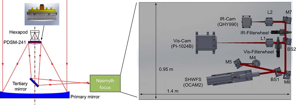
    Fig. 1. The sketch of the 1.8-m adaptive telescope.
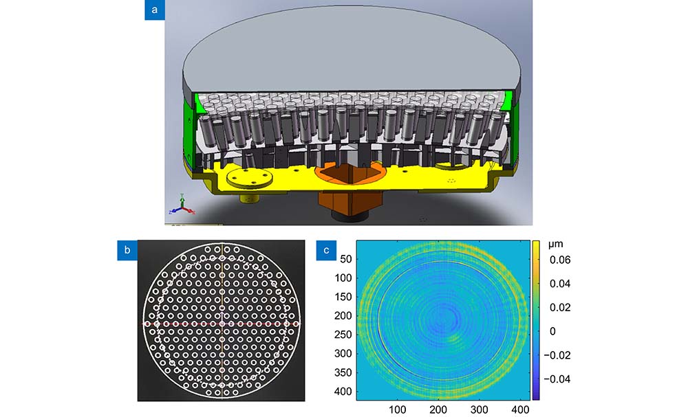
    (a) The sketch of the PDSM-241. (b) Actuator layout (clear aperture: 270 mm). (c) The uncompensated aberration of PDSM-241.
    Fig. 2. (a) The sketch of the PDSM-241. (b) Actuator layout (clear aperture: 270 mm). (c) The uncompensated aberration of PDSM-241.
    The sub-aperture layout of the SHWFS (effective diameter: 16 mm) and the image of a collimated wave.
    Fig. 3. The sub-aperture layout of the SHWFS (effective diameter: 16 mm) and the image of a collimated wave.
    Control strategy of the AOS.
    Fig. 4. Control strategy of the AOS.
    (a) Flowchart of calibration of the interaction matrix. (b) Closed-loop wavefront control.
    Fig. 5. (a) Flowchart of calibration of the interaction matrix. (b) Closed-loop wavefront control.
    Temporal high order RMS error with AO system on and off at the time (UT) 14:00 on April 28, 2022. (HIP–49669, altitude angle: 71 degrees, azimuth: 217 degrees).
    Fig. 6. Temporal high order RMS error with AO system on and off at the time (UT) 14:00 on April 28, 2022. (HIP–49669, altitude angle: 71 degrees, azimuth: 217 degrees).
    Residual wavefront error distribution at the time (UT) between 13:30 and 16:15 on April 28, 2022.
    Fig. 7. Residual wavefront error distribution at the time (UT) between 13:30 and 16:15 on April 28, 2022.
    Closed-loop wavefront noise error distribution at the time (UT) between. 13:30 and 16:15 on April 28, 2022.
    Fig. 8. Closed-loop wavefront noise error distribution at the time (UT) between. 13:30 and 16:15 on April 28, 2022.
    Image motion comparison with the AO system on and off. x-tilt: Open-loop: 0.4", Closed-loop: 0.015" (left panel); y-tilt: Open-loop: 0.21", Closed-loop: 0.017" (right panel)
    Fig. 9. Image motion comparison with the AO system on and off. x-tilt: Open-loop: 0.4", Closed-loop: 0.015" (left panel); y-tilt: Open-loop: 0.21", Closed-loop: 0.017" (right panel)
    PSD of tracking error in open-loop and closed-loop with the AO system on and off. x-tilt (left panel) and y-tilt (right panel).
    Fig. 10. PSD of tracking error in open-loop and closed-loop with the AO system on and off. x-tilt (left panel) and y-tilt (right panel).
    PSD of AO system in open-loop and closed-loop (left panel), error transfer function (right panel).
    Fig. 11. PSD of AO system in open-loop and closed-loop (left panel), error transfer function (right panel).
    Comparison of the Zernike RMS error in open-loop (circle) and closed-loop (square). The solid curve is the fitting of the Kolmogorov turbulence model to the open-loop data.
    Fig. 12. Comparison of the Zernike RMS error in open-loop (circle) and closed-loop (square). The solid curve is the fitting of the Kolmogorov turbulence model to the open-loop data.
    The distribution of r0 at the time (UT) between 13:51 and 14:08 on April 28, 2022.
    Fig. 13. The distribution of r0 at the time (UT) between 13:51 and 14:08 on April 28, 2022.
    The visible short exposure images of the star HIP49669 (2022-04-28), the images are displayed in linear scale and the peaks are normalized to 1. (a) R-band, SR=0.491, FWHM = 0.0937”. (b) R-band, SR=0.481, FWHM = 0.0953”. (c) I-band, SR=0.574, FWHM=0.113”. (d) I-band, SR = 0.582, FWHM=0.111”.
    Fig. 14. The visible short exposure images of the star HIP49669 (2022-04-28), the images are displayed in linear scale and the peaks are normalized to 1. (a) R-band, SR=0.491, FWHM = 0.0937”. (b) R-band, SR=0.481, FWHM = 0.0953”. (c) I-band, SR=0.574, FWHM=0.113”. (d) I-band, SR = 0.582, FWHM=0.111”.
    Comparison of I-band closed-loop (left) and open-loop (right) image of the star HIP63418 (V-magnitude: 8.16).
    Fig. 15. Comparison of I-band closed-loop (left) and open-loop (right) image of the star HIP63418 (V-magnitude: 8.16).
    R band (~640 nm) closed-loop Strehl ratios with guide stars of different magnitudes.
    Fig. 16. R band (~640 nm) closed-loop Strehl ratios with guide stars of different magnitudes.
    I band (~860 nm) closed-loop Strehl ratios with guide stars of different magnitudes.
    Fig. 17. I band (~860 nm) closed-loop Strehl ratios with guide stars of different magnitudes.
    SystemParameterValue
    Visible imagingWavelength600~1000 nm (R, I)
    CameraPI 1024B
    Pixel FoV0.04 arcsec
    Size1024×1024
    Table 0. Main parameters of the Imaging cameras.
    ParameterValue
    Wavelength (nm)400–600
    Effective diameter (mm)16
    Number of pixels in a sub-aperture14×14
    Field of view (arcsec)14
    Pixel size (µm)24
    Frame rate (Hz)Up to 2000
    Pixel Format240×240
    Microlens array15×17
    Table 0. Main parameters of the SHWFS.
    ParameterValue
    Reflecting surfaceConvex hyperboloid
    Spacing (mm)19.3
    Number of actuators241
    Maximum stroke (µm)±6
    Actuator configurationTriangle
    Clear aperture (mm)270
    Coupling10%
    Weight (kg)15
    Table 0. Details about the PDSM-241.
    MagnitudeFrame rate (Hz) (WFS)Tracking accuracy (") (AO-off)Tracking accuracy (") (AO-on)Higher-order RMS (nm) (AO-off)Higher-order RMS (nm) (AO-on)Closed-loop wavefront noise RMS (nm)
    0.420000.51880.0387348.788.17.5
    1.3620000.45060.0323304.772.312.3
    2.1420000.44200.0236251.873.015.3
    2.8920000.70810.0520329.687.124.8
    4.2420000.59500.0543293.692.042.4
    5.0120000.60650.0528323.5112.052.9
    6.0320000.53240.0433360.0100.0112.4
    7.1512000.55180.0736300.7145.8141.2
    8.165000.47580.1178308.0190.4176.2
    9.521500.34110.2331317.9243.1235.9
    Table 0. The performance of the adaptive telescope with different magnitudes.
    Youming Guo, Kele Chen, Jiahui Zhou, Zhengdai Li, Wenyu Han, Xuejun Rao, Hua Bao, Jinsheng Yang, Xinlong Fan, Changhui Rao. High-resolution visible imaging with piezoelectric deformable secondary mirror: experimental results at the 1.8-m adaptive telescope[J]. Opto-Electronic Advances, 2023, 6(12): 230039
    Download Citation