Adaptive optics systems (AOSs) are widely used in astronomical telescopes for static and dynamic wavefront compensation^1-6. The fundamental principle involved is to change at least one surface of AOS mirrors in real time to adapt the wavefront of the input light. The AOS has been developed for over 70 years and has two crucial research fields. One is to improve it by novel signal processing techniques⁷, while the other is to merge it into the telescope. Traditionally, AOS is installed at the post-focus of a telescope, independent of the telescope optics. Special deformable mirrors (including tip-tilt mirrors) and relay optics are usually required, resulting in a complex imaging system with low throughput and high heat dissipation. The innovative proposal, first introduced by Beckers⁸, involves integrating the telescope and AOS through the concept of deformable secondary mirror (DSM), which is also called adaptive secondary mirror (ASM). The multiple mirror telescope (MMT)⁹ was the first DSM-based telescope, following the large binocular telescope (LBT)¹⁰, Magellan telescope (MT)^{11, 12} and the UT4 of the very large telescope (VLT)¹³. These large-diameter adaptive telescopes were all based on the voice-coil DSMs (VCDSMs). These telescopes have successfully demonstrated the advantages of DSMs, such as high optical throughput, compact volume, and wavefront correction for different foci. In the context of medium-aperture telescopes, we first demonstrated the feasibility of piezoelectric DSM (PDSM) in 2016 for astronomical observation. We developed a 73-actuator PDSM and used it in the 1.8-m telescope for on-sky experiment^{14, 15}. The structure of the PDSM is much simpler than the VCDSM, in which no additional position sensor, local electronics or active thermal control is required. However, the main drawback of PDSM is its relatively limited stroke compared to the VCDSM, measuring about ±6 µm in our cases. Another medium-aperture telescope using a DSM is the University of Hawaii's 88-inch telescope on Mauna Kea¹⁶. TNO and its partners are developing a 204-actuator DSM for the ground layer adaptive optics system of the telescope. The actuator of this DSM is based on the electromagnetic hybrid variable reluctance that can bring a stroke of 35 µm (PV) and an inter-act stroke of 4.5 µm. Three 30-m class telescopes will be built in the near future, significantly impacting astronomical observation. The 39-m European Extremely Large Telescope will use M4 as the deformable mirror and M3 as the tip-tilt mirror while the 24-m Great Magellan Telescope will directly use VCDSMs¹⁷ following the success of LBT, MT, and others. The adaptive telescope has become a cutting-edge concept that more and more astronomical telescopes would adopt. Besides the adaptive telescope concept, the visible diffraction-limited imaging brought by the DSM has also been investigated recently. The LBT and MT teams have made a lot of efforts and demonstrated the superior advantages of DSM for visible imaging^{18, 19}.

Given the advantages of large-aperture telescopes, we want to investigate the concept of medium-aperture adaptive telescopes. In this paper, we present an introduction to the PDSM-based adaptive telescope, especially with the new high-order DSM called PDSM-241. We also present its application in the 1.8-m telescope that can perform near-diffraction-limited imaging in the visible region. Section System overview addresses the system overview, and the on-sky performance is presented in Section Performance. Finally, we conclude and discuss in Section Conclusions.

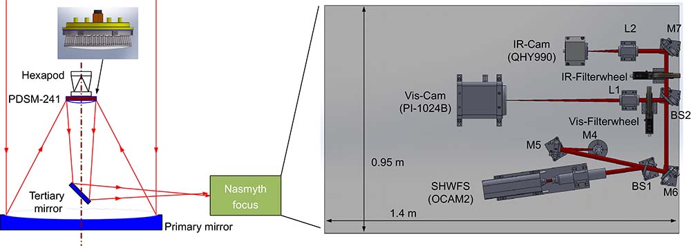
The 1.8-m adaptive telescope is described in detail in Fig. 1. The PDSM-241 is mounted on a hexapod, and this combined setup effectively functions as the wavefront correction system. No other wavefront corrector is required anymore. The atmospheric turbulence distorts the light from stars, which is then collected by the primary mirror. After reflecting from the primary mirror, the wavefront aberration of the light is compensated by the PDSM-241 and the hexapod and then reflected by the tertiary mirror towards the Nasmyth focus. Other instruments of the telescope can also use the PDSM-241 for wavefront compensation just by rotating the tertiary mirror and reflecting the light to other foci.

In the Nasmyth focus, the light is firstly reflected by the M4 to make it parallel to the optical platform and then collimated by the off-axis parabolic mirror M5. The collimated light with a diameter of 16 mm is firstly split by the BS1, where most visible light goes into the Shack-Hartmann wavefront sensor (SHWFS) while the residual light passes through BS1, and then is reflected by M6. The beam-splitter BS2 splits the residual light into two parts where L1 focuses the visible light into the visible camera “Vis-Cam,” and the infrared light is reflected by M7 and focused by the L2 into the infrared Camera “IR-Cam”. Two filter wheels are used for the selection of different imaging bands. At present, the IR Cam has not yet been installed.

Details regarding the PDSM-241 are provided in Table 1. PDSM-241 is equipped with a mirror of 320 mm diameter made of quartz. The clear aperture of PDSM-241 is about 270 mm and is driven by 241 piezoelectric actuators to change its surface for wavefront correction. The maximum stroke of deformation is ±6 µm. Given the convex hyperboloid profile of PDSM-241, a focus is absent prior to its integration into the telescope. It has brought some challenges in calibrating the interaction matrix between the PDSM-241 and the SHWFS. All 241 actuators were used for wavefront compensation. The coupling of neighboring actuators was about 10.0%. No defective actuator has been found up to now. The mechanical structure of the PDSM-241 is shown in Fig. 2(a), and the layout of the actuators is present in Fig. 2(b). The uncompensated aberration of PDSM-241 is presented in Fig. 2(c) with root mean square (RMS) wavefront error less than 10 nm. It is crucial for visible diffraction-limited imaging.

The SHWFS has a 15×17 sub-aperture configuration to sample the pupil with a total of 192 sub-apertures excluding 7 obscured sub-apertures in the center²⁰ as shown in Fig. 3. The equivalent spacing of sub-apertures on the primary mirror was about 11.7 cm which was close to the Fried parameter of the central wavelength λs=500 nm in the SHWFS under good seeing condition in Lijiang Observatory. The camera of the SHWFS was the OCAM2S EMCCD produced by the First Light Company with a pixel format of 240×240. The maximum sampling frequency of the camera was 2000 Hz. This specification was enough in the design of the real-time controller (RTC). The field of view (FoV) for each pixel was approximately 1 arcsecond, while a sub-aperture had a FoV of 14 arcsec. The details about this SHWFS are summarized in Table 2.

The control mechanism for our system is shown in Fig. 4. The primary control for closed-loop work was based on a leaky integrator. The voltages were directly reconstructed from the measured slopes with a reconstruction matrix obtained by the truncated SVD algorithm. A condition number of 10 was set to balance the accuracy and robustness. No special tip-tilt mirror was used to simplify the system structure as much as possible. Additionally, the tracker was based on the combination of the hexapod and the PDSM-241. Tip-tilt with low frequency was corrected by the hexapod with a framerate of about 1 Hz, while the PDSM handled high-frequency correction at a frame rate of 2000 Hz, particularly suitable for bright stars. The other aberrations were all compensated by the PDSM-241. We took advantage of the relatively large stroke of the PDSM-241 for the 1.8-m telescope. The stroke is usually large enough for tracking and high-order correction needs. The calibration of the interaction matrix is of great importance for AOS. Traditionally, this is done on an optical platform by perfect artificial sources. However, in our cases, making such an artificial source upstream of the PDSM was too complex or impossible. Therefore, we took the bright natural guide star as an alternative. However, atmospheric turbulence and telescope vibration can adversely affect the calibration. Vibration or other tracking errors may induce a random global shift in the sub-aperture spots, potentially displacing them toward the edges and causing confusion with the actuator's response. We dealt with this problem using two procedures. First, the hexapod was controlled to correct the tip-tilt in order to keep the spots in the central area of the sub-aperture before initiating the PDSM. In this scenario, the hexapod operates in a closed loop, while the PDSM operates in an open loop. Second, the global tilt was removed from the actuator's response. The second procedure may have little impact on the accuracy of the interaction matrix. However, since the global tilt produced by a single actuator is minimal, we can neglect it without a noticeable effect on the correction performance. Besides, the PDSM can still correct the global-tilt when all actuators are used to fit the global-tilt with the influence functions measured by the interferometer. The turbulence aberration is often random and it can be effectively rejected by the combination of push-pull and Hadamard. The push-pull can reduce the static or low-frequency aberrations while the Hadamard's averaging effect can suppress the high-frequency aberrations. As first time reported by Kasper²¹, the interaction matrix calibration error of the Hadamard method is as follows:

(EEt)Hadamard=n−1vm−2(NNt),（1）

where n is the dimension of the Hadamard matrix, vm is the driving voltage, and N is the slope measurement error caused by turbulence or noise. In our case, n was set as 256, and vm was set to 0.3 V in order to avoid WFS saturation. The variance of the slope measurement error was averaged by 256 in our experiment.

The interaction matrix calibration and closed-loop wavefront control processes are shown in Fig. 5.

Both visible and infrared cameras were used in this study. The visible channel had a filter wheel that could be switched between the R and I band. Moreover, while the infrared channel had another filter wheel that can be switched between the J and H band. The details of the infrared camera are currently unavailable. In contrast, the details of the visible imaging system are shown in Table 3. The visible camera has already been installed while the infrared camera will be installed soon.

PDSM241-AO was designed to provide the wavefront correction capability required by visible imaging. We have done some on-sky experiments to demonstrate it. This section presents the experimental results obtained during March and April of 2022.

The AOS is controlled with Zernike modes, and the number of modes to be compensated depends on the SHWFS and PDSM. Although the PDSM has 241 actuators, the normalized fitting errors estimated by the influence functions indicate that some modes larger than 135 may have poor fitting capability. Thus, for the RMS value of dynamic wavefront error, the first 135-order Zernike modes were compensated by the PDSM in this AO system. Except for tip-tilt, we analyzed the aberrations of the other 133 higher-order Zernike modes in the time domain, considering only the effects of dynamic turbulence. We used a star with a magnitude of 1.36 as an example. The atmospheric coherence length at that time was about 10.9 cm. As shown in Fig. 6, when the AO system is in closed-loop, the RMS value of the dynamic wavefront error for a star is significantly reduced. Moreover, the higher-order aberration caused by dynamic turbulence is effectively suppressed. Specifically, the RMS value of the dynamic wavefront error decreased from about 304.7 nm to 72.3 nm on average when the AO system was turned on. Additionally, the static aberration of the optical system was corrected from 368.7 nm to 35.1 nm using the RMS value. Without loss of generality, we also analyzed the closed-loop performance over a period of time. Figure 7 depicts the distribution of high-order closed-loop wavefront errors, which are mostly below 100 nm. The closed-loop wavefront noise error can be estimated by analyzing the high-frequency part of the power spectral density (PSD) of the Zernike modes which is dominated by noise. We can calculate the closed-loop noise variance by the integral of the noise PSD. Figure 8 presents the histogram of closed-loop wavefront noise RMS errors, most of which are below 10 nm.

As discussed earlier, PDSM241-AO uses the combination of the hexapod and PDSM241 to do the tracking. The tracking error is first measured by the SHWFS and then sent to the RTC for controlling the combination. The tracking error in the time domain of a star is shown in Fig. 9. It describes that after the system is in a closed loop, whether in the x-tilt or the y-tilt, the temporal behavior of the tilt error is effectively smaller. Moreover, the x-tilt is reduced by a factor of 26.7, and the y-tilt is reduced by a factor of 12.4. For clarity of this experiment, Fig. 10 depicts the PSDs of the x-tilt and y-tilt in open and closed loops. Furthermore, by analyzing the intersection of these two PSD curves in the frequency domain, we can roughly estimate that the error rejection bandwidth is about 75 Hz. Given that the sampling frequency of the SHWFS is set to 2000 Hz, the bandwidth corresponds to approximately 1/25 of this frequency value. At the same time, there are apparent narrow-band vibrations at 6 Hz and 50 Hz in the x-tilt and near 50 Hz in the y-tilt. The integrators have made certain compensation for it, and the tracking accuracy can still meet the needs of the 1.8-m adaptive telescope.

Concerning the high-order correction, a modal control method was applied. The PSDs of the 3^rd, 35^th, 65^th, and 135^th Zernike modes with AO-on and AO-off are listed in the left part of Fig. 11. The corresponding error transfer function curves are shown on the right side of Fig. 11. The selection of these four modes is mainly to summarize the correction effect of the system from different modes in order to cover different spatial frequencies in the first 135 modes. From the PSD curves we can infer the level of the measurement noise (flat curve past 600 Hz) as well as estimate the turbulence power distribution (−8/3 exponent). Furthermore, the error rejection bandwidth of the AO system can be estimated to be around 85 Hz based on the position where the error transfer function curve intersects with 0 dB.

The atmospheric coherence length at that time was estimated by analyzing the variance of the Zernike modal coefficients from the 3^rd to the 15^th using Kolmogorov turbulence theory. Firstly, the Zernike modal coefficient matrix was reconstructed from the open-loop slope matrix measured by SHWFS. Then, according to the ordering and normalization scheme proposed by Noll²², the wavefront error Δ was estimated by the variance of these thirteen Zernike coefficients (3^rd to the 15^th). Finally, the atmospheric coherence length r0 was calculated by the following relation.

Δavg=(D/r0)5/3,（2）

here Δavg indicates the average wavefront error, and D represents the telescope aperture. The rationale for excluding the first two Zernike modes is to mitigate measurement errors stemming from vibration, and the higher Zernike modes (>15) are also omitted to minimize modal coupling and aliasing errors. Figure 12 compares open-loop and closed-loop Zernike mode RMS error and the Kolmogorov turbulence fitting result under two atmospheric turbulence environments. All Zernike modes are apparently well compensated. In Fig. 13, a statistical analysis of the Fried parameter r0 is presented for the time duration (UT) between 13:51 and 14:08 on April 28, 2022. It shows that r0 values during this period are around 12 cm at the 500 nm wavelength.

One of the most critical advantages of an adaptive telescope is its high throughput, achieved by using considerably fewer mirrors than traditional optical telescopes. A higher limiting magnitude is anticipated. In the subsequent discussion, we present details of the system's performance with different guide stars from the SHWFS data and closed-loop images. Table 4 lists the frame rate, tracking accuracy, higher-order aberration, and RMS value of closed-loop wavefront noise error for observations conducted on stars ranging from magnitude zero to nine. For star magnitudes brighter than magnitude 6 the loop can be closed at the maximum frame rate, but for magnitudes dimmer than magnitude 6 the frame rate must be reduced to obtain acceptable performances.

Owing to the effective closed-loop correction of the DSM, high-resolution images were captured by the proposed adaptive telescope. Some of the closed-loop visible images at R and I bands are shown in Fig. 14. The pixel scale of the visible camera was about 0.0397 arcsec after calibrating it by a double star. This star, HIP37279, is a bright star of V-magnitude 0.4. The elevation when the star was observed was about 42 degrees. The average seeing during the observation of this star was estimated to be approximately 0.86", determined by analyzing the slopes recorded by the SHWFS just after the closed-loop correction.

One of the most significant advantages of the adaptive telescope concept is its high optical throughput. We checked its performance on some faint guide stars. In order to facilitate visible imaging, small-scale sub-apertures were designed, approximately 11.7 cm in size, when mapped to the primary mirror. This size is much smaller than large-scale adaptive telescopes such as LBT, Magellan, or VLT. The number of sub-apertures remained unchanged compared to telescopes with pyramid WFS. As a result, the limiting magnitude was based on the 192-sub-aperture configuration for the 1.8-m telescope. The open and closed-loop I-band images for a star with a V-magnitude of 8 are shown in Fig. 15. The peak intensity is clearly improved.

On the night of 2022-04-28, many closed-loop images were captured to characterize the performance of our adaptive telescope. Several stars with V-magnitudes from 0 to 8 were observed. The closed-loop performances are displayed in Fig. 16 and Fig. 17. When the V-magnitude is brighter than 7, the adaptive telescope can work at a frequency of 2000 Hz, which is the maximum frequency of the OCAM2. The error rejection bandwidth remains constant, with performance primarily influenced by the prevailing seeing conditions. In most cases, the Strehl ratios at the R band are larger than 0.2. Similarly, closed-loop images with Strehl ratios of about 0.4 at the I band can be observed. For a star of magnitude 7, the adaptive telescope can work at 1000 Hz. For a star of magnitude higher than 8, the frame rate of the SHWFS is reduced to 500 Hz, resulting in noticeable performance degradation.

To upgrade a 1.8-m telescope into an adaptive telescope, a 241-actuator PDSM was developed and integrated into it. Because of the adaptive telescope concept, the structure of this telescope was straightforward, and the number of mirrors was also small, leading to high optical throughput. The system was robust as the SHWFS and imaging cameras were all on the Nasmyth foci, and no pupil shift correction was required. The wavefront correctors comprised a PDSM for high-order wavefront correction and a hexapod, combining both for tracking purposes. On-sky experiments were carried out using this adaptive telescope with diffraction-limited visible and infrared imaging. The performance of this adaptive telescope for stars with different V-magnitudes was evaluated. The limiting magnitude was high enough considering the high-density configuration of the sub-apertures. In general, the PDSM was demonstrated to be a perfect choice for building an adaptive telescope with a diameter of ~2 m. Experiments will be done to investigate the PDSM's applications in large and medium aperture (~4 m) telescopes, especially for visible diffraction-limited imaging.

References

[1] CH Rao, NT Gu, XJ Rao, C Li, LQ Zhang et al. First light of the 1.8-m solar telescope–CLST. Sci China Phys Mech Astron, 109631(2020).
[3] CH Rao, L Zhu, LQ Zhang, XJ Rao, H Bao et al. Development of solar adaptive optics. Opto-Electron Eng, 170733(2018).
[4] CH Rao, L Zhu, XJ Rao, LQ Zhang, H Bao et al. Instrument description and performance evaluation of a high-order adaptive optics system for the 1m new vacuum solar telescope at Fuxian solar observatory. Astrophys J, 210(2016).
[5] JY Wang, YM Guo, L Kong, LQ Zhang, NT Gu et al. Automatic disturbance identification for linear quadratic Gaussian control in adaptive optics. Mon Not R Astron Soc, 5126-5138(2020).
[6] D Kim, H Choi, T Brendel, H Quach, M Esparza et al. Advances in optical engineering for future telescopes. Opto-Electron Adv, 210040(2021).
[7] YM Guo, LB Zhong, L Min, JY Wang, Y Wu et al. Adaptive optics based on machine learning: a review. Opto-Electron Adv, 200082(2022).
[8] JM Beckers. Adaptive optics for astronomy: principles, performance, and applications. Annu Rev Astron Astrophys, 13-62(1993).
[9] FP Wildi, G Brusa, M Lloyd-Hart, LM Close, A Riccardi. First light of the 6.5-m MMT adaptive optics system. Proc SPIE, 17-25(2003).
[10] S Esposito, A Riccardi, E Pinna, A Puglisi, F Quirós-Pacheco et al. Large binocular telescope adaptive optics system: new achievements and perspectives in adaptive optics. Proc SPIE, 814902(2011).
[11] KM Morzinski, LM Close, JR Males, D Kopon, PM Hinz et al. MagAO: Status and on-sky performance of the Magellan adaptive optics system. Proc SPIE, 914804(2014).
[12] R Briguglio, F Quirós-Pacheco, JR Males, M Xompero, A Riccardi et al. Optical calibration and performance of the adaptive secondary mirror at the Magellan telescope. Sci Rep, 10835(2018).
[14] YM Guo, A Zhang, XL Fan, CH Rao, L Wei et al. First on-sky demonstration of the piezoelectric adaptive secondary mirror. Opt Lett, 5712-5715(2016).
[15] YM Guo, A Zhang, XL Fan, CH Rao, L Wei et al. First light of the deformable secondary mirror-based adaptive optics system on 1.8m telescope. Proc SPIE, 99091D(2016).
[16] S Kuiper, WA Jonker, MP Maniscalco, H Priem, C Coolen et al. Adaptive secondary mirror development for the UH-88 telescope. In 6th International Conference on Adaptive Optics for Extremely Large Telescopes(2019).
[17] S Hippler. Adaptive optics for extremely large telescopes. J Astron Instrum, 1950001(2019).
[18] F Pedichini, M Stangalini, F Ambrosino, A Puglisi, E Pinna et al. High contrast imaging in the visible: first experimental results at the Large Binocular Telescope. Astron J, 74(2017).
[19] LM Close, JR Males, K Morzinski, D Kopon, K Follette et al. Diffraction-limited visible light images of orion trapezium cluster with the magellan adaptive secondary adaptive optics system (MagAO). Astrophys J, 94(2013).
[20] YM Guo, Y Wu, Y Li, XJ Rao, CH Rao. Deep phase retrieval for astronomical Shack–Hartmann wavefront sensors. Mon Not R Astron Soc, 4347-4354(2022).
[21] M Kasper, E Fedrigo, DP Looze, H Bonnet, L Ivanescu et al. Fast calibration of high-order adaptive optics systems. J Opt Soc Am A, 1004-1008(2004).
[22] RJ Noll. Zernike polynomials and atmospheric turbulence. J Opt Soc Am A, 207-211(1976).