First-photon imaging via a hybrid penalty

Xiao Peng; Xin-Yu Zhao; Li-Jing Li; Ming-Jie Sun

doi:10.1364/PRJ.381516

Abstract

First-photon imaging is a photon-efficient, computational imaging technique that reconstructs an image by recording only the first-photon arrival event at each spatial location and then optimizing the recorded photon information. The optimization algorithm plays a vital role in image formation. A natural scene containing spatial correlation can be reconstructed by maximum likelihood of all spatial locations constrained with a sparsity regularization penalty, and different penalties lead to different reconstructions. The

l_{1}

-norm penalty of wavelet transform reconstructs major features but blurs edges and high-frequency details of the image. The total variational penalty preserves edges better; however, it induces a “staircase effect,” which degrades image quality. In this work, we proposed a hybrid penalty to reconstruct better edge features while suppressing the staircase effect by combining wavelet

l_{1}

-norm and total variation into one penalty function. Results of numerical simulations indicate that the proposed hybrid penalty reconstructed better images, which have an averaged root mean square error of 12.83%, 5.68%, and 10.56% smaller than those of the images reconstructed by using only wavelet

l_{1}

-norm penalty, total variation penalty, or recursive dyadic partitions method, respectively. Experimental results are in good agreement with the numerical ones, demonstrating the feasibility of the proposed hybrid penalty. Having been verified in a first-photon imaging system, the proposed hybrid penalty can be applied to other noise-removal optimization problems.

1. INTRODUCTION

Single-photon counting is an important technique for scene detection under long-distance or weak illumination conditions [1–4]. Whenever the detector senses a photon arrival event after the object is illuminated by a laser pulse, the number of counting increases by one. However, photon detection is not necessarily triggered by every laser pulse, but rather it is a statistical event that is related to many aspects. Besides the illumination energy, the detector quantum efficiency, and the propagation loss, the detection probability $p$ of a photon arrival event being detected, which is calculated as the ratio between the number of detected photons $m$ and the number of emitted laser pulses $l$ , is mainly proportional to the reflectivity of an object. The problem of single-photon counting is that even as the detector has the capability to sense a single photon, it needs to accumulate a large number of photon arrival events to obtain different reflectivity information of different spatial locations of a scene.

First-photon imaging [5,6] addressed this problem by recording only the first-photon arrival event and the number of illumination pulses $k$ required at each spatial location of the scene. Theoretically, $1 / k$ contains the information of photon detection probability $p$ as well; however, due to its statistical nature, it contains a random noise because $k ≪ l$ . Given a certain a priori knowledge of the scene, the random noise at different spatial locations can be suppressed by optimization algorithms, and the image of the scene can be reconstructed by suppressing the noise for all spatial locations. Usually, the noise is described as Poisson [5–8] when the scene is illuminated by a pulsed laser, and it can be suppressed by minimizing the weighted sum of the negative log-likelihood and a sparsity penalty constraint for all spatial locations of the scene [5].

The spatial correlation of a natural scene is usually described in certain transform domains, such as discrete wavelet transformation and total variation (TV) [9–12]. In the wavelet domain, the coefficients of a natural scene image contain only a few large values while the rest are close to zero. Therefore, the $l_{1}$ -norm of the wavelet coefficients can be used as a penalty constraint for noise suppression optimization [13]. The $l_{1}$ -norm of the wavelet coefficients penalty constraint is referred to as the $l_{1}$ -norm hereafter. Unfortunately, the coefficients of both high-frequency details, such as edges, and noise of the reconstructed image are also large in the wavelet domain; consequently, noise having frequencies similar to the details cannot be suppressed by applying the $l_{1}$ -norm penalty directly [14,15]. Alternatively, the TV norm reflects the smoothness of the image’s gradient, which is essentially the $l_{1}$ -norm of the derivatives [16]. The TV norm represents the sparsity of the gradient of the image [10,17], and denoising of a reconstructed image can be performed by minimizing the TV norm as a penalty constraint [10,18–20]. However, TV regularization causes a “staircase effect” [21] that severely degrades the image fidelity. Therefore, while different sparsity penalty constraints suppress the noise of the reconstructed image, they also induce different side effects, jeopardizing the quality of the reconstructed image.

Sign up for Photonics Research TOC. Get the latest issue of Photonics Research delivered right to you！Sign up now

In this work, we address the problem by introducing a hybrid penalty constraint, which combines the $l_{1}$ -norm and the TV norm, to balance the noise suppression and the induced side effects and to improve the quality of the reconstructed images. Compared to the images independently reconstructed by the $l_{1}$ -norm or TV, the images reconstructed using the proposed hybrid penalty demonstrate better qualities in both numerical simulations and experiments. The proposed hybrid penalty combining the $l_{1}$ -norm and TV norm is referred to as $l_{1}$ -TV hereafter.

2. PRINCIPLE OF $l_{1}$ -TV PENALTY-BASED IMAGE RECONSTRUCTION ALGORITHM

Compared to conventional photon counting imaging schemes, first-photon imaging greatly reduces the number of photons needed to be detected by recording only the number of transmitted pulses when the first photon arrival event is detected at each spatial location [5,6]. However, if the image is reconstructed using only maximum likelihood estimation based on the probability model of photon detection, severe random noises exist in the reconstructed image. Taking advantage of the spatial correlation in the natural scenes, i.e., adjacent spatial locations having strong correlations can be captured via sparse coefficients of the discrete wavelet transform, the mathematical model of these random noises can be approximately viewed as a convex optimization problem, which can be solved numerically and efficiently. Here, a new hybrid penalty is proposed for the convex optimization algorithm of first-photon imaging, and its principle is given as follows.

A. Pixelwise Reflectivity Maximum Likelihood Estimation

The statistical model of returning photons for each spatial location in the first-photon imaging process obeys the Poisson distribution. When a discrete spatial location ( $i$ , $j$ ) is illuminated by a laser pulse, the probability of no photon detected is [22] $p_{0} (i, j) = e^{- γ (f_{i, j} S + B T_{r})},$ (1)where $γ$ is the detection efficiency, $f_{i, j}$ denotes scene reflectivity at the spatial location ( $i$ , $j$ ), and $S$ is the average photon number in the reflected signal received from a single laser pulse illuminating a unity-gray-scale spatial location, defined as $S = \int_{0}^{T_{r}} s (t) d t$ . $s (t)$ is the intensity-modulated laser pulse shape function. The Gaussian laser pulse waveform is chosen in this paper. $B$ denotes the arrival rate of background photons at the detector; $T_{r}$ is the pulse repetition period. Because each transmitted pulse gives rise to one independent photon detection event, the probability of the first-photon detection at the $n_{i, j}$ th transmitted pulse obeys the geometric distribution in Eq. (2): $p_{r} [n_{i, j} = k] = p_{0} {(i, j)}^{k - 1} [1 - p_{0} (i, j)], for k = 1, 2 \dots .$ (2)Using the second-order Taylor series approximation of Eq. (2) with the assumption that $γ (S f_{i, j} + B T_{r}) ≪ 1$ , a negative log-likelihood function, which relates the reflectivity of the scene to the counts of transmitted pulses, can be given as $F (f_{i, j} | n_{i, j}) = (γ S f_{i, j} + B T_{r}) (n_{i, j} - 1) - \log [γ (S f_{i, j} + B T_{r})] .$ (3)Given the constraint of nonnegative reflectivity, the pointwise maximum likelihood estimation of $f_{i, j}$ is $f_{i, j}^{0} = \max [\frac{1}{(n_{i, j} - 1) γ S} - \frac{B_{T r}}{S}, 0] .$ (4)

B. Sparsity Penalties of the Image Reconstruction

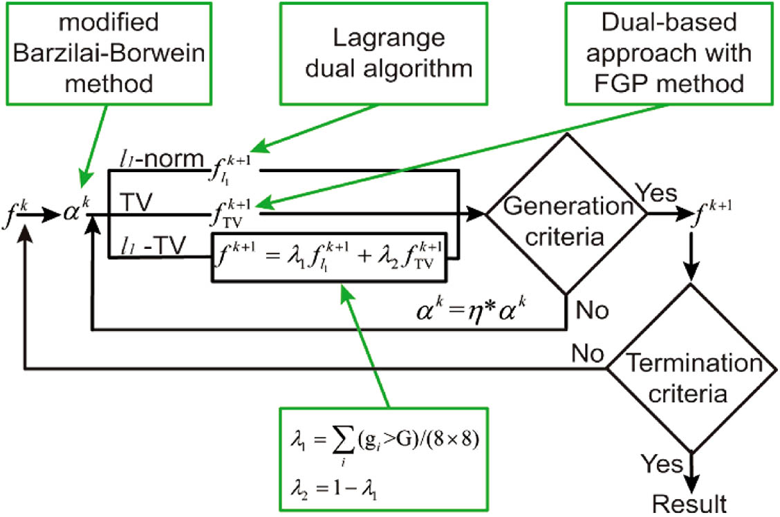
It is necessary to select a penalty term to constrain the sparsity of the underlying image over the transform domain. The reflectivity estimation $f^{'}$ is an optimization problem that consists of a probabilistic statistical model and a sparse penalty, $f^{'} = argmin \sum_{i}^{n} \sum_{j}^{n} F (f_{i, j} | n_{i, j}) + τ p e n (f) subject to f_{i, j} \geq 0, for all i, j,$ (5)where $p e n (\cdot)$ is the selected sparsity penalty constraint and $τ$ is a weighing factor indicating how strictly the penalty will be applied. We solve this optimization problem using the SPIRAL algorithm [9,23–26]. For one generation of the optimization, Eq. (5) can be rewritten into Eq. (6) via separable approximation [22]: $f^{k + 1} = \underset{f \in R^{n}}{argmin} ϕ^{k} (f) = \underset{f \in R^{n}}{argmin} \frac{1}{2} {‖ f - s^{k} ‖}_{2}^{2} + \frac{τ}{α^{k}} p e n (f), f \geq 0, s^{k} = f^{k} - \frac{1}{α^{k}} \nabla F (f^{k}) .$ (6)The generation stops when $f^{k + 1}$ satisfies the criterion $ϕ (f^{k + 1}) \leq \max_{i = {[k - M]}_{+, \dots k}} ϕ (f^{i}) - \frac{σ α^{k}}{2} {‖ f^{k + 1} - f^{k} ‖}_{2}^{2},$ (7)where the initial value of $α^{k}$ is chosen using a modified Barzilai–Borwein method [27] and safeguarded to be within the range $[α_{\min}, α_{\max}]$ . Its value will be repeatedly increased by a factor $η$ until the solution satisfies Eq. (7), $M$ is a nonnegative integer, and $σ \in (0, 1)$ is a small constant.

The $l_{1}$ -norm and TV can be used as penalty function in Eq. (5) [9]. The $l_{1}$ -norm suppresses the noise but blurs the edges as well. The TV penalty enhances the edge features but also induces the staircase effect. In this work, we propose a hybrid penalty that combines the $l_{1}$ -norm and TV with weighting parameters. The reflectivity estimation is performed by Eq. (8), $f^{'} = argmin \sum_{i}^{n} \sum_{j}^{n} F (f_{i, j} | n_{i, j}) + τ ({‖ θ ‖}_{1} + μ {‖ f ‖}_{TV}),$ (8)where $θ = W^{T} f$ are the expansion coefficients of the discrete wavelet transform, $μ$ is a weighting constant to balance the asymmetry between the two penalties, and ${‖ f ‖}_{TV}$ is described in Eq. (9), ${‖ f ‖}_{TV} = \sum_{i}^{n - 1} \sum_{j}^{n} | f_{i, j} - f_{i + 1, j} | + \sum_{i}^{n} \sum_{j}^{n - 1} | f_{i, j} - f_{i, j + 1} | .$ (9)The weighted sum of these convex functions, being either smooth convex, such as negative log-likelihood and the $l_{1}$ -norm, or nonsmooth such as the TV, can be solved via convex optimization.

In each generation, we solve Eq. (6) with $τ p e n (f) = τ ({‖ θ ‖}_{1} + μ {‖ f ‖}_{TV})$ via three steps.

Step 1. Fixing the TV term, the problem of Eq. (8) becomes a minimization problem, which can be solved by solving its Lagrangian dual, i.e., SPIRAL- $l_{1}$ [9]: $θ_{l_{1}}^{k + 1} = \underset{θ \in R^{n}}{argmin} ϕ^{k} (θ) = \underset{θ \in R^{n}}{argmin} \frac{1}{2} {‖ θ - s^{k} ‖}_{2}^{2} + \frac{τ}{α^{k}} {‖ θ ‖}_{1}, subject to W θ \geq 0 .$ (10)

Step 2. Fixing the $l_{1}$ -norm term, the problem of Eq. (8) becomes a TV-regularized problem, which can be solved via a dual approach with a fast gradient projection method [9,18]: $f_{TV}^{k + 1} = \underset{f \in R^{n}}{argmin} ϕ^{k} (f) = \underset{f \in R^{n}}{argmin} \frac{1}{2} {‖ f - s^{k} ‖}_{2}^{2} + \frac{τ}{α^{k}} {‖ f ‖}_{TV}, subject to f \geq 0 .$ (11)

Step 3. The final gray-scale image is the weighted sum of $f_{l_{1}}$ and $f_{TV}$ as Eq. (12): $f^{k + 1} = λ_{1} f_{l_{1}}^{k + 1} + λ_{2} f_{TV}^{k + 1},$ (12)where weighting factors $λ_{1}$ and $λ_{2}$ are used to balance the denoise effects of the $l_{1}$ -norm and the TV during reconstruction. The values of $λ_{1}$ and $λ_{2}$ are determined by the smoothness of the image after each iteration. Particularly, in order to consider both the global and local smoothness of the reconstructed image, we divide the image into $8 \times 8$ sections and calculate the average of the adjacent pixel gradients of each small section $g_{i}$ and the average of the adjacent pixel gradients of the whole image $G$ . The more complex structure of the image, the smaller the number of $g_{i} > G$ . Therefore, we define $λ_{1} = \sum_{i} (g_{i} > G) / (8 \times 8)$ ; and $λ_{2} = 1 - λ_{1}$ .

The schematics of the SPIRAL algorithm using the $l_{1}$ -norm, TV, and $l_{1}$ -TV are illustrated in Fig. 1. The starting reflectivity image $f^{(0)}$ of the optimization is the maximum likelihood estimation of the recorded first-photon information. Steps 1–3 are repeated for each generation till Eq. (7) is satisfied. The termination criterion for the whole optimization is $| ϕ^{k + 1} - ϕ^{k} | / ϕ^{k} \leq tolp .$ (13)It is worth mentioning that the $l_{1}$ -TV method is proposed with the aim of balancing the noise suppression and the induced side effects of the $l_{1}$ -norm and the TV, and it is difficult to strictly prove its convergence. Other algorithms with a stronger theoretical convergence guarantee, such as the alternating direction method of multipliers (ADMM)-based method [28], could be used to solve the convex optimization here. Nevertheless, in Fig. 2, the mean square error (MSE) term of error function $ϕ^{k} (f)$ in Eq. (6) is plotted versus the number of optimization generations, showing that the proposed hybrid $l_{1}$ -TV has a similar convergence profile to the $l_{1}$ -norm and the TV. A recent work of parallel proximal algorithm also presented a similar observation for hybrid regularization [29].

SPIRAL algorithm using the l1-norm, TV, and l1-TV. FGP, fast gradient projection.

Figure 1.SPIRAL algorithm using the $l_{1}$ -norm, TV, and $l_{1}$ -TV. FGP, fast gradient projection.

Figure 2.MSE convergence profiles of the $l_{1}$ -norm, TV, and $l_{1}$ -TV.

3. EXPERIMENTAL RESULTS

To evaluate the performance of the SPIRAL optimization algorithm based on different penalties, i.e., the $l_{1}$ -norm, TV, and $l_{1}$ -TV, a group of 35 general images, which are pictures of general objects or scenes, are used in numerical simulations. Taking one image as an example, the first-photon detection process based on the geometric distribution of the transmitted pulse counts is simulated independently for each transverse spatial location of the scene image. The counts of the transmitted pulses and the arrival times of the single photon consist of the first-photon information of the image. The maximum likelihood estimation of the first-photon information is retrieved numerically to be the starting reflectivity image $f^{(0)}$ , and the SPIRAL optimization algorithm is then performed until Eq. (13) is satisfied. The root mean square error (RMSE) between the reconstructed image and the ground truth is calculated to evaluate the quality of the reconstructed image as $RMSE = \sqrt{\frac{\sum_{i = 1}^{m} \sum_{j = 1}^{n} {(f_{i, j} - f_{i, j}^{'})}^{2}}{m \times n}},$ (14)where $m$ and $n$ are the dimensions of the image, and $f_{i, j}$ and $f_{i, j}^{'}$ are the gray scale at the spatial location ( $i$ , $j$ ) of the reconstructed image and ground truth.

For each image, the optimization is performed 3 times, with the $l_{1}$ -norm, the TV, and the $l_{1}$ -TV being the penalty function each time. For the $l_{1}$ -norm and $l_{1}$ -TV penalty, a typical wavelet basis, DB-6 basis [9], is chosen for wavelet transform. For numerical simulations, we set $γ = 0.08$ , $S = 0.02$ , $B T_{r} = 0.001$ , $η = 2$ , $σ = 0.1$ , $M = 10$ , $μ = 0.333$ , and $α_{\min} = 1 / α_{\max} = 1 \times 10^{- 3}$ . $τ$ in Eq. (5) is chosen from ${0.1, 0.2, \dots, 1}$ for each image individually to guarantee that the RMSE of the resulting image is minimized. tolp in Eq. (13) is set to $1 \times 10^{- 4}$ , which guarantees that the optimization converges well. It is worth mentioning that some parameters, such as detection efficiency $γ$ and pulse repetition rate $T_{r}$ , are directly related to the specification of the experimenting devices, while other parameters, such as average reflected photon number $S$ , step factor $η$ , and penalty weighting constant $μ$ , depend on the illumination condition as well as the structure of the image. These parameters can be estimated automatically via methods of different sophistications [30,31]. In this work, weighting factors $λ_{1}$ and $λ_{2}$ of the proposed hybrid penalty are automatically estimated; other parameters are either given or manually tuned for optimal reconstruction.

For comparison, a cycle-spun translation-invariant version of recursive dyadic partitions method (RDP-Ti) [9,32] is also performed during our simulations. Furthermore, many other penalties, such as nonlocal low-rank [33,34] and tensor decomposition [35], can be used to solve the minimization problem of Eq. (6). However, in this work, the major focus is on the $l_{1}$ -norm and the TV, which is closely related to the proposed hybrid $l_{1}$ -TV penalty; results yielded by RDP-Ti are also provided for comparison.

The RMSEs of all resulting images reconstructed via the four methods are given in Fig. 3. Thirty images, out of all 35, reconstructed with the $l_{1}$ -TV have the smallest RMSE, compared to those yielded by the $l_{1}$ -norm, the TV or the RDP-Ti. The averaged RMSE of the 35 images reconstructed by the $l_{1}$ -TV penalty is 0.0881, which is 12.83%, 5.68%, and 10.56% smaller than those of the images reconstructed by the $l_{1}$ -norm, the TV, and the RDP-Ti, respectively, demonstrating that the proposed $l_{1}$ -TV hybrid penalty effectively improves the quality of the reconstructed images. It is worth mentioning that the $l_{1}$ -norm reconstructs images with the smallest RMSEs in 2 cases where the ground truths have high-frequency details similar to noise. The TV also yields the best quality images in another 3 cases where the original images contain larger blocky areas so that staircase effect does not degrade the reconstruction quality much. These demonstrate the reconstruction features using the $l_{1}$ -norm and TV penalties and support the proposition of the hybrid $l_{1}$ -TV penalty in the purpose of balancing the reconstruction features of the $l_{1}$ -norm and the TV.

Figure 3.RMSEs of the reconstructed images using the $l_{1}$ -norm (green square), TV (blue diamond), RPD-Ti (purple dot), and $l_{1}$ -TV (red triangle).

Samples of resulting images are illustrated in Fig. 4. Different reconstruction features yielded using the $l_{1}$ -norm, TV, RDP-Ti, and $l_{1}$ -TV can be observed from the corresponding columns. The TV works better with smooth images (drawer and sofa), while the $l_{1}$ -norm is superior for a complex image (church). The images reconstructed by the $l_{1}$ -TV, which preserves certain high-frequency details while reducing the staircase effect, have the smallest RMSEs for all three sample groups, in comparison to those of the $l_{1}$ -norm, the TV, and the RDP-Ti reconstruction results.

Figure 4.Comparison of three groups of reconstructed images using different penalties. From left to right are ground truth (GT), $l_{1}$ -norm, TV, RDP-Ti, and $l_{1}$ -TV. The RMSEs between the reconstructed images and their corresponding ground truth are listed below, respectively.

Interestingly, the first-photon imaging technique captures not only 2D images but 3D structures. The convex optimization algorithm for depth information reconstruction is very similar to that of reflectivity reconstruction. Only the negative log-likelihood function of Eq. (3), which relates the reflectivity to the counts of transmitted pulses, is replaced with another negative log-likelihood function, now relating the depth to the arrival time of the first counted photon. The details of the algorithm can be found in the supplementary material of Ref. [5]. Here, the proposed hybrid $l_{1}$ -TV penalty is also applied to reconstruct the depth information of a scene. The reconstructed results using different methods are illustrated in Fig. 5. Because the scene, being three planes with a 5 mm interval between the adjacent two, has a simple structure, the performances of the TV and $l_{1}$ -TV are much better than those of the $l_{1}$ -norm and RDP-Ti.

Figure 5.Comparison of reconstructed depth information using different penalties. From left to right are ground truth (GT), $l_{1}$ -norm, TV, RDP-Ti, and $l_{1}$ -TV. The RMSEs between the reconstructions and the ground truth are listed below, respectively.

An experiment is performed to further verify the feasibility of the proposed $l_{1}$ -TV penalty. The experimental system schematic is shown in Fig. 6. Instead of a scanning galvo in the experimental system of Ref. [5], here, a digital micromirror device (Texas Instruments Discovery 4100, spatial resolution $1024 \times 768$ , operating at 10 kHz modulation rate), illuminated by a pulsed laser (PicoQuant LDH-P-635, average power 5.2 mW, 80 MHz repetition rate), is used to raster-scan the object using a $128 pixel \times 128 pixel$ resolution. The information of the first photon detection event of each scanned spatial location is recorded by a photomultiplier tube (PicoQuant PMA Hybrid 07, time resolution $< 50 ps$ ) and the time-correlated single-photon counting module (PicoQuant HydraHarp400, time bin 1 ps), the latter of which is synchronized with the pulsed laser. The raw first-photon data are then transferred to a computer for image reconstruction using the process described in Section 2.

Figure 6.Schematic of experimental system. A repetitive pulsed laser is modulated by a digital micromirror device (DMD) and raster-scans the object pixel by pixel. The reflected photons from the object arrive at a photomultiplier tube (PMT) and trigger a photon-arrival event according to the photon detection probability. The first-photon data are then recorded by a time-correlated single-photon counting (TCSPC) module and transferred to a computer for image reconstruction.

To provide a reference image for the calculation of RMSE, an image captured by conventional photon counting is given in Fig. 7. For the photon-counting image, the averaged photon counts and corresponding illumination laser pulses per pixel are 43 counts and 8000 pulses, respectively, satisfying the photon-starved condition for time-correlated single-photon detection. Contrarily, for the first-photon image, the averaged numbers are 1 count and 202 pulses per pixel. First-photon imaging shows approximately 40 times better energy efficiency over conventional photon-counting imaging. The images reconstructed using different penalties are shown in Fig. 7. Both visual observation and calculated RMSEs indicate that the proposed hybrid $l_{1}$ -TV penalty yields images with better qualities than the other three methods do. The experimental results are in good agreement with those of the numerical simulation, indicating the feasibility of the proposed method.

Figure 7.Comparison of experimental results yielded by different approaches. From left to right are photon counting (PC), $l_{1}$ -norm, TV, RDP-Ti, and $l_{1}$ -TV. The RMSEs between the reconstructed images and the photon counting image are listed below, respectively.

Like numerical simulation, another experiment is performed to reconstruct the depth information of a scene. In this experiment, the object in Fig. 6 is replaced with a simple 3D structure, which consists of three flat surfaces with a 5 mm interval between the adjacent two. The depth information reconstructed using different methods is shown in Fig. 8. RMSEs calculated between the ground truth and the reconstructed depth indicate that the proposed hybrid $l_{1}$ -TV penalty retrieves more accurate depth information than the other three methods do.

Figure 8.Comparison of experimentally reconstructed depth information using different penalties. From left to right are ground truth (GT), $l_{1}$ -norm, TV, RDP-Ti, and $l_{1}$ -TV. The RMSEs between the reconstructions and the ground truth are listed below, respectively.

4. CONCLUSION

In summary, the characteristics of noise suppression using the $l_{1}$ -norm- or TV-based convex optimization for first-photon image are analyzed. In order to overcome the side effects induced by the two penalties during the optimization, a hybrid penalty combining the $l_{1}$ -norm and the TV is proposed to be applied to the image reconstruction algorithm. Results of numerical simulations show that the averaged RMSE of 35 images reconstructed by the $l_{1}$ -TV penalty is 12.83%, 5.68%, and 10.56% smaller than those of the images reconstructed by the $l_{1}$ -norm, the TV, and the RDP-Ti, respectively. The experimental results are in good agreement with the numerical ones, further demonstrating the feasibility of the proposed $l_{1}$ -TV penalty. The effectiveness of the proposed hybrid $l_{1}$ -TV penalty is also verified in depth information reconstruction, both numerically and experimentally. The work presented here mainly focuses on first-photon imaging. However, the proposed method can also be applied to solve other Poisson noise problems caused by photon detection, such as fluorescence microscopy.

References

[1] A. McCarthy, R. J. Collins, N. J. Krichel, V. Fernández, A. M. Wallace, G. S. Buller. Long-range time-of-flight scanning sensor based on high-speed time-correlated single-photon counting. Appl. Opt., 48, 6241-6251(2009).

[2] M. S. Oh, H. J. Kong, T. H. Kim, S. E. Jo, B. W. Kim, D. J. Park. Development and analysis of a photon-counting three-dimensional imaging laser detection and ranging (ladar) system. J. Opt. Soc. Am. A, 28, 759-765(2011).

[3] W. J. He, B. Y. Sima, Y. F. Chen, H. D. Dai, Q. Chen, G. H. Gu. A correction method for range walk error in photon counting 3D imaging LIDAR. Opt. Commun., 308, 211-217(2013).

[4] D. Shin, F. Xu, D. Venkatraman, D. Lussana, F. Zappa, V. K. Goyal, F. N. C. Wong, J. H. Shapiro. Photon-efficient computational imaging with a single-photon camera. Nat. Commun., 7, 12046(2016).

[5] A. Kirmani, D. Venkatraman, D. Shin, A. Colaço, F. N. C. Wong, J. H. Shapiro, V. K. Goyal. First-photon imaging. Science, 343, 58-61(2014).

[6] X. Liu, J. Shi, X. Wu, G. H. Zeng. Fast first-photon ghost imaging. Sci. Rep., 8, 5012(2018).

[7] D. Shin, A. Kirmani, A. Colaço, V. K. Goyal. Parametric Poisson process imaging. Proceedings of the IEEE Global Conference on Signal and Information Processing, 1053-1056(2013).

[8] A. Colac, A. Kirmani, G. A. Howland, J. C. Howell, V. K. Goyal. Compressive depth map acquisition using a single photon-counting detector: parametric signal processing meets sparsity. Proceedings of the IEEE Conference on Computer Vision and Pattern Recognition, 96-102(2012).

[9] Z. T. Harmany, R. F. Marcia, R. M. Willett. This is spiral-tap: sparse Poisson intensity reconstruction algorithms-theory and practice. IEEE Trans. Image Process., 21, 1084-1096(2012).

[10] Y. Kang, L. F. Li, X. J. Duan, T. Y. Zhang, D. J. Li, W. Zhao. Photon-limited depth and reflectivity imaging with sparsity regularization. Opt. Commun., 392, 25-30(2017).

[11] D. Shin, A. Kirmani, V. K. Goyal, J. H. Shapiro. Computational 3D and reflectivity imaging with high photon efficiency. IEEE International Conference on Image Processing, 46-50(2014).

[12] D. Shin, A. Kirmani, V. K. Goyal, J. H. Shapiro. Photon-efficient computational 3D and reflectivity imaging with single-photon detectors. IEEE Trans. Comput. Imaging, 1, 112-125(2015).

[13] A. Kirmani, D. Venkatraman, A. Colac, F. N. C. Wong, V. K. Goyal. High photon efficiency computational range imaging using spatio-temporal statistical regularization. CLEO: QELS_Fundamental Science, QF1B.2(2013).

[14] S. Mallat, A. Wavelet. Tour of Signal Processing(1998).

[15] S. Ruikar, D. D. Doye. Image denoising using wavelet transform. International Conference on Mechanical and Electrical Technology, 509-515(2010).

[16] L. I. Rudin, S. Osher, E. Fatemi. Nonlinear total variation based noise removal algorithms. Physica D, 60, 259-268(1992).

[17] Y. Kang, Y. P. Yao, Z. H. Kang, L. Ma, T. Y. Zhang. Performance analysis of compressive ghost imaging based on different signal reconstruction techniques. J. Opt. Soc. Am. A, 32, 1063-1067(2015).

[18] A. Beck, M. Teboulle. Fast gradient-based algorithms for constrained total variation image denoising and deblurring problems. IEEE Trans. Image Process., 18, 2419-2434(2009).

[19] M. A. T. Figueiredo, R. D. Nowak, S. J. Wright. Gradient projection for sparse reconstruction: application to compressed sensing and other inverse problems. IEEE J. Sel. Top. Signal Process., 1, 586-597(2008).

[20] A. Chambolle. An algorithm for total variation minimization and applications. J. Math. Imaging Vis., 20, 89-97(2004).

[21] J. Xu, X. Feng, Y. Hao, Y. Han. Image decomposition and staircase effect reduction based on total generalized variation. J. Syst. Eng. Electron., 25, 168-174(2014).

[22] D. L. Snyder. Random point processes. J. Roy. Stat. Soc., 139, 990(1975).

[23] Z. T. Harmany, R. F. Marcia, R. M. Willett. SPIRAL out of convexity: sparsity-regularized algorithms for photon-limited imaging. Proc. SPIE, 7533, 75330R(2010).

[24] R. F. Marcia, Z. T. Harmany, R. M. Willett. Compressive coded apertures for high-resolution imaging. Proc. SPIE, 7723, 75330R(2010).

[25] J. C. Emmanuel, M. B. Wakin, S. P. Boyd. Enhancing sparsity by reweighted l₁ minimization. J. Fourier Anal. Appl., 14, 877-905(2008).

[26] S. J. Wright, R. D. Nowak, M. A. T. Figueiredo. Sparse reconstruction by separable approximation. IEEE Trans. Image Process., 57, 2479-2493(2009).

[27] J. Barzilai, J. M. Borwein. Two-point step size gradient methods. IMA J. Numer. Anal., 8, 141-148(1988).

[28] R. Nishihara, L. Lessard, B. Recht, A. Packard, M. I. Jordan. A general analysis of the convergence of ADMM. Proceedings of the International Conference on Machine Learning, 343-352(2015).

[29] N. Pustelnik, C. Chaux, J. C. Pesquet. Parallel proximal algorithm for image restoration using hybrid regularization. IEEE Trans. Image Process., 20, 2450-2462(2011).

[30] S. Ramani, T. Blu, M. Unser. Monte-Carlo sure: a black-box optimization of regularization parameters for general denoising algorithms. IEEE Trans. Image Process., 17, 1540-1554(2008).

[31] Y. Altmann, S. McLaughlin, M. Padgett. Unsupervised restoration of subsampled images constructed from geometric and binomial data. Proceedings of the IEEE Computational Advances in Multi-Sensor Adaptive Processing, 1521-1525(2017).

[32] R. M. Willett, R. D. Nowak. Multiscale Poisson intensity and density estimation. IEEE Trans. Inf. Theory, 53, 3171-3187(2007).

[33] W. S. Dong, G. M. Shi, X. Li, Y. Ma, F. Huang. Compressive sensing via nonlocal low-rank regularization. IEEE Trans. Image Process., 23, 3618-3632(2014).

[34] W. S. Dong, G. M. Shi, X. Li. Nonlocal image restoration with bilateral variance estimation: a low-rank approach. IEEE Trans. Image Process., 22, 700-711(2012).

[35] B. Recht, M. Fazel, P. A. Parrilo. Guaranteed minimum-rank solutions of linear matrix equations via nuclear norm minimization. SIAM Rev., 52, 471-501(2010).