
Na Zhang, Chenglong Wang, Fei Liang, Guodong Zhu, Lei Zhao. Characteristics of Energy Flux Distribution of Concentrating Solar Power Systems[J]. Laser & Optoelectronics Progress, 2018, 55(12): 120004
- Laser & Optoelectronics Progress
- Vol. 55, Issue 12, 120004 (2018)
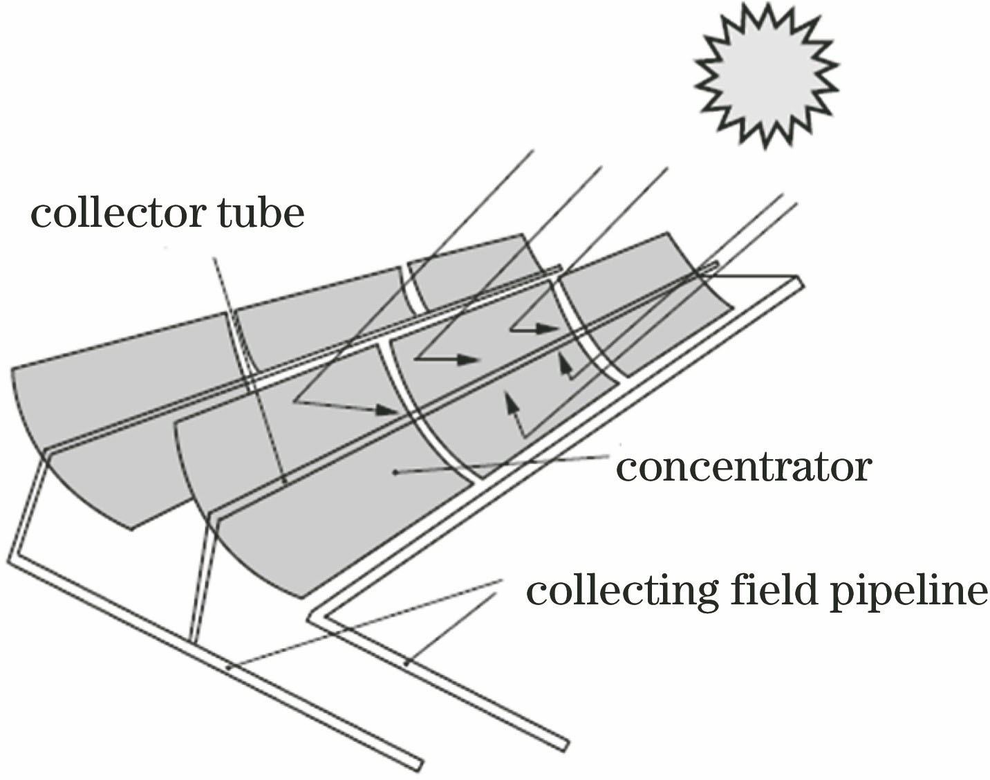
Fig. 1. Schematic of the condensation in parabolic trough system
![Non-uniform flux distribution of the absorber tubes measured by CTM method[12]](/richHtml/lop/2018/55/12/120004/img_2.jpg)
Fig. 2. Non-uniform flux distribution of the absorber tubes measured by CTM method[12]
Fig. 3. Collector with ParaScan-II[13]
Fig. 4. Flux distribution on the surface of bend absorber[19]
Fig. 5. Flux distribution on the outer surface of absorber[21]
Fig. 6. Comparison of flux distribution between the MCRT method and Jeter’s method[22]
Fig. 7. Heat flux distributions on parabolic trough receiver[23]
Fig. 8. Temperature distribution on the outer surface of absorber tube[23]. (a) Contour plot; (b) temperature versus coordinate Y
Fig. 9. Comparison of flux distribution between MACM method and the method proposed by Jeter and He[24]
Fig. 10. Trough receiver with secondary reflector[34]
Fig. 11. Radiation path and irradiance distribution of the VFPT concentrator on the receiver[35]
Fig. 12. Trough condenser system with homogenized reflectors[36]. (a) Schematic of structure; (b) light path
Fig. 13. Comparison between conventional parabolic trough collector and parabolic trough collector with homogenizing reflector[36]
Fig. 14. Linear Fresnel concentrating system layout
Fig. 15. Schematic of evacuated tube and CPC
Fig. 16. Light path of CPC cavity receiver[41]
Fig. 17. Relative radiation intensity distribution of the collector tube[41]
Fig. 18. Flux distribution on the absorber and CPC[45]
Fig. 19. Circumferential temperature distribution on absorber[45]
Fig. 20. Flux distribution of linear Fresnel absorber with different incidence angles. (a) 45°; (b) 60°; (c) 75°; (d) 90°
Fig. 21. Geometric structure of a winged secondary reflector[47]
Fig. 22. Radial distribution on wing receiver[47]
Fig. 23. Profiles of SPC[48]
Fig. 24. Flux distribution of different target lines in SPC configuration[48]
Fig. 25. Surface flux distribution on the absorber of systems with three typical reflectors three types of reflector system[49]
Fig. 26. Flux distribution corresponding to five kinds of scattered sight lines[50]
Fig. 27. Influence of surface error on the flux distribution of collector tube[49]
Fig. 28. Simple diagram of tower collection system
Fig. 29. Heliostat
Fig. 30. Beam PHLUX diagram on tubular receiver[53]
Fig. 31. Solar flux distribution on the aperture of cavity receiver[65]
Fig. 32. Distribution of surface flux in cavity receiver[66]
Fig. 33. Solar flux distribution in the porous absorber of volumetric receiver[67]
Fig. 34. Heat flux distribution at different receiver mounting height[67]
Fig. 35. Optimized fluid flow layout for receiver[69]
Fig. 36. Temperature distribution on the outer surface of receivers with or without porous insert[70]
Fig. 37. Optimal distribution of energy flux density after the receiver surface optimization[65]
Fig. 38. Comparison of solar flux distributions on inner surfaces of cavity receiver[73]. (a) 1 aiming point; (b) 21 aiming points
Fig. 39. Cavity receiver wall temperature distribution under different depth[75]. (a) 0; (b) 1.0 m; (c) 2.0 m; (d) 3.0 m
Fig. 40. Schematic of dish light collecting system light
Fig. 41. Flux distribution on absorbing surfaces for different cavity receivers in solar dish system[84]. (a) Cylindrial; (b) dome; (c) heteroconical; (d) ellipse; (e) spherical; (f) conic
Fig. 42. Cavity absorber surface of dish system[85]. (a) Radiation flux distribution; (b) temperature profile of the inner surface
Fig. 43. Solar flux density in focal plane[24]. (a) Comparison and confirmation; (b) distributed cloud map
Fig. 44. Sketch of shape pattern of upside-down pear cavity receiver[87]
Fig. 45. Comparison of solar flux distribution on receiver surface between spherical receiver and pear-like receiver[87]
Fig. 46. Cavity receiver with flat convex quartz glass[88]
Fig. 47. Comparison of solar flux distribution of three hemisphere receivers in solar dish system[88]
Fig. 48. Schematic of plane mirror array

Set citation alerts for the article
Please enter your email address
© Copyright 2018-2021 | Chinese Laser Press. All Rights Reserved 沪ICP备15018463号-20