• Photonics Research
  • Vol. 9, Issue 12, 2332 (2021)
Kunkun Wang1、2, Lei Xiao1, Wei Yi3、4、6, Shi-Ju Ran5、7, and Peng Xue1、*
Author Affiliations
  • 1Beijing Computational Science Research Center, Beijing 100084, China
  • 2School of Physics and Optoelectronics Engineering, Anhui University, Hefei 230601, China
  • 3CAS Key Laboratory of Quantum Information, University of Science and Technology of China, Hefei 230026, China
  • 4CAS Center for Excellence in Quantum Information and Quantum Physics, Hefei 230026, China
  • 5Department of Physics, Capital Normal University, Beijing 100048, China
  • 6e-mail: wyiz@ustc.edu.cn
  • 7e-mail: sjran@cnu.edu.cn
  • show less
    DOI: 10.1364/PRJ.434217 Cite this Article Set citation alerts
    Kunkun Wang, Lei Xiao, Wei Yi, Shi-Ju Ran, Peng Xue. Experimental realization of a quantum image classifier via tensor-network-based machine learning[J]. Photonics Research, 2021, 9(12): 2332 Copy Citation Text show less
    Illustration of the main steps of implementing the TN-based quantum classifier. In steps (i)–(iii), we map the images of N=784 pixels (features) to quantum states and train the matrix product state (MPS) classifier using these images in the MNIST dataset by a supervised learning algorithm. The MPS consists of N tensors represented by squares, with the label index represented by a flag. We calculate the entanglement entropies of the MPS and retain only N˜=3 or 5 features with the largest entanglement entropies. Then, we train a reduced MPS with the N˜ retained features. In steps (iv) and (v), the reduced MPS is translated to a circuit acting on N˜ qubits and further to a circuit using the qubit-efficient scheme, which involves N˜′=2 qubits and N˜ gates, including a single-qubit gate U1 and N˜−1 two-qubit gates Ui (i=2, 3 or i=2,…,5). We employ two schemes to implement the classifier, whose orders of operations are indicated by the red and blue arrows, respectively.
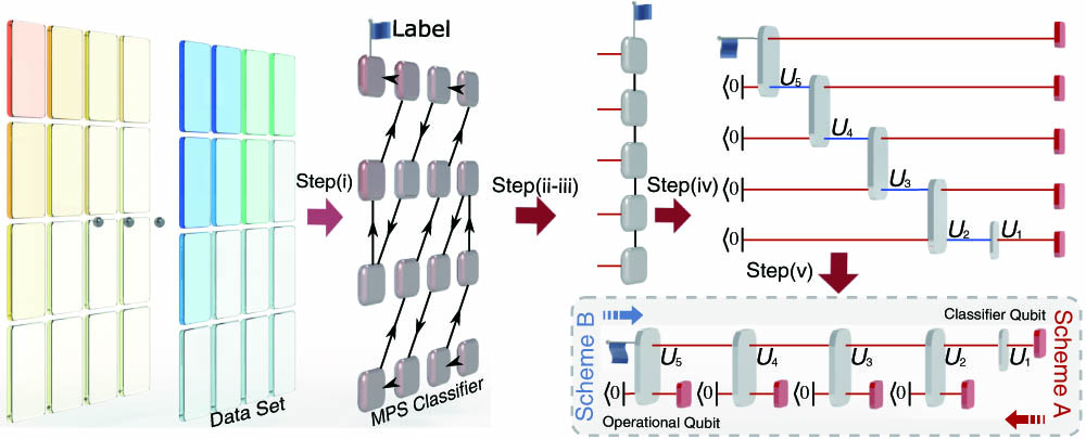
    Fig. 1. Illustration of the main steps of implementing the TN-based quantum classifier. In steps (i)–(iii), we map the images of N=784 pixels (features) to quantum states and train the matrix product state (MPS) classifier using these images in the MNIST dataset by a supervised learning algorithm. The MPS consists of N tensors represented by squares, with the label index represented by a flag. We calculate the entanglement entropies of the MPS and retain only N˜=3 or 5 features with the largest entanglement entropies. Then, we train a reduced MPS with the N˜ retained features. In steps (iv) and (v), the reduced MPS is translated to a circuit acting on N˜ qubits and further to a circuit using the qubit-efficient scheme, which involves N˜=2 qubits and N˜ gates, including a single-qubit gate U1 and N˜1 two-qubit gates Ui (i=2,  3 or i=2,,5). We employ two schemes to implement the classifier, whose orders of operations are indicated by the red and blue arrows, respectively.
    Training and testing accuracies of classifying the “0” and “1” digits in the MNIST dataset as functions of N˜. Data are obtained by averaging the accuracies over 20 numerical simulations, and error bars indicate the statistical uncertainty.
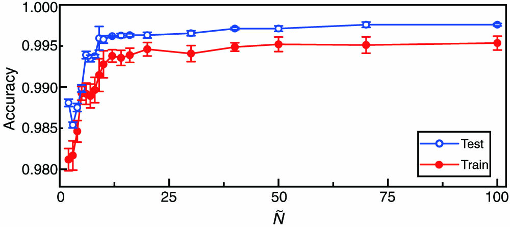
    Fig. 2. Training and testing accuracies of classifying the “0” and “1” digits in the MNIST dataset as functions of N˜. Data are obtained by averaging the accuracies over 20 numerical simulations, and error bars indicate the statistical uncertainty.
    Experimental demonstration of quantum classifier with the three-layer construction. For each pair of photons generated by spontaneous parametric down conversion, one photon serves as the trigger, and the other, the signal photon, proceeds through the experimental setup corresponding to the two schemes. Under Scheme A, the signal photon is projected onto the polarization state |ψ1⟩ of the classifier qubit via a PBS and an HWP H0. It is then sent through an interferometric network, composed of HWPs and BDs, before being detected by APDs in coincidence with the trigger photon. The single-qubit gate U1 is realized by an HWP, and two-qubit gates U2 and U3 are realized by BDs and HWPs. The input states |ψ2⟩ and |ψ3⟩ are encoded in the spatial modes of photons and prepared via the HWPs (H1, H2, H9, and H10) in controlled beam splitters (CBSs), which, by combining the spatial and polarization degrees of freedom, effectively expand the dimension of the system. A 1 m long single-mode fiber serves as a spatial filter in between successive modules of the two-qubit gate, and a set of wave plates is introduced to offset the impact of the fiber on the photon polarizations. For detection, photons are projected onto the upper spatial mode |u⟩ by discarding those in the lower one, and a projective measurement of σz is realized through an HWP, a PBS, and APDs. Scheme B is the exact reverse process of Scheme A, where photons are sent into the setup through the output port of Scheme A.
    Fig. 3. Experimental demonstration of quantum classifier with the three-layer construction. For each pair of photons generated by spontaneous parametric down conversion, one photon serves as the trigger, and the other, the signal photon, proceeds through the experimental setup corresponding to the two schemes. Under Scheme A, the signal photon is projected onto the polarization state |ψ1 of the classifier qubit via a PBS and an HWP H0. It is then sent through an interferometric network, composed of HWPs and BDs, before being detected by APDs in coincidence with the trigger photon. The single-qubit gate U1 is realized by an HWP, and two-qubit gates U2 and U3 are realized by BDs and HWPs. The input states |ψ2 and |ψ3 are encoded in the spatial modes of photons and prepared via the HWPs (H1, H2, H9, and H10) in controlled beam splitters (CBSs), which, by combining the spatial and polarization degrees of freedom, effectively expand the dimension of the system. A 1 m long single-mode fiber serves as a spatial filter in between successive modules of the two-qubit gate, and a set of wave plates is introduced to offset the impact of the fiber on the photon polarizations. For detection, photons are projected onto the upper spatial mode |u by discarding those in the lower one, and a projective measurement of σz is realized through an HWP, a PBS, and APDs. Scheme B is the exact reverse process of Scheme A, where photons are sent into the setup through the output port of Scheme A.
    Theoretical results of the testing set under the (a) three- and (b) five-layer constructions, respectively. The output states are shown in the x−z plane of the Bloch sphere associated with the classifier qubit. The green squares (blue triangles) indicate successful recognition of the hand-written digit “0” (“1”). Red symbols indicate cases in which the classifier fails to recognize the image.
    Fig. 4. Theoretical results of the testing set under the (a) three- and (b) five-layer constructions, respectively. The output states are shown in the xz plane of the Bloch sphere associated with the classifier qubit. The green squares (blue triangles) indicate successful recognition of the hand-written digit “0” (“1”). Red symbols indicate cases in which the classifier fails to recognize the image.
    Experimental classification of images within the testing set. Measured probabilities of the projective measurements on output states of quantum classifiers with the (a) three- and (b) five-layer constructions. Left, Scheme A; right, Scheme B. Colored bars represent experimental results, while hollow bars represent their theoretical predictions. Error bars indicate the statistical uncertainty, obtained by assuming Poissonian statistics in the photon-number fluctuations. (c) The classification results for eight typical hand-written digits in the testing set. Rows represent the index of images, namely the hand-written digits, the experimental and theoretical probability differences, and classification results. P0,13 and P0,15 represent probabilities associated with the three- and five-layer constructions, respectively.
    Fig. 5. Experimental classification of images within the testing set. Measured probabilities of the projective measurements on output states of quantum classifiers with the (a) three- and (b) five-layer constructions. Left, Scheme A; right, Scheme B. Colored bars represent experimental results, while hollow bars represent their theoretical predictions. Error bars indicate the statistical uncertainty, obtained by assuming Poissonian statistics in the photon-number fluctuations. (c) The classification results for eight typical hand-written digits in the testing set. Rows represent the index of images, namely the hand-written digits, the experimental and theoretical probability differences, and classification results. P0,13 and P0,15 represent probabilities associated with the three- and five-layer constructions, respectively.
    Classification of images outside the MNIST dataset. (a) Measured probabilities of the output states of quantum classifiers. (b) Classification results.
    Fig. 6. Classification of images outside the MNIST dataset. (a) Measured probabilities of the output states of quantum classifiers. (b) Classification results.
    Experimental demonstration of quantum classifier under Scheme B (three-layer construction). The classifier and operational qubits are initialized in |H⟩⊗|u⟩ or |V⟩⊗|u⟩ via a PBS and an HWP. After each gate operation Ui† (i=1, 2, 3), a projective measurement |ψi⟩⟨ψi| is performed on the operational qubit via a CBS. This is the reverse process of the setup in Fig. 1 of the main text.
    Fig. 7. Experimental demonstration of quantum classifier under Scheme B (three-layer construction). The classifier and operational qubits are initialized in |H|u or |V|u via a PBS and an HWP. After each gate operation Ui (i=1,2,  3), a projective measurement |ψiψi| is performed on the operational qubit via a CBS. This is the reverse process of the setup in Fig. 1 of the main text.
    Kunkun Wang, Lei Xiao, Wei Yi, Shi-Ju Ran, Peng Xue. Experimental realization of a quantum image classifier via tensor-network-based machine learning[J]. Photonics Research, 2021, 9(12): 2332
    Download Citation