Experimental realization of a quantum image classifier via tensor-network-based machine learning

Kunkun Wang; Lei Xiao; Wei Yi; Shi-Ju Ran; Peng Xue

doi:10.1364/PRJ.434217

Abstract

Quantum machine learning aspires to overcome intractability that currently limits its applicability to practical applications. However, quantum machine learning itself is limited by low effective dimensions achievable in state-of-the-art experiments. Here, we demonstrate highly successful classifications of real-life images using photonic qubits, combining a quantum tensor-network representation of hand-written digits and entanglement-based optimization. Specifically, we focus on binary classification for hand-written zeroes and ones, whose features are cast into the tensor-network representation, further reduced by optimization based on entanglement entropy and encoded into two-qubit photonic states. We then demonstrate image classification with a high success rate exceeding 98%, through successive gate operations and projective measurements. Although we work with photons, our approach is amenable to other physical realizations such as nitrogen-vacancy centers, nuclear spins, and trapped ions, and our scheme can be scaled to efficient multi-qubit encodings of features in the tensor-product representation, thereby setting the stage for quantum-enhanced multi-class classification.

1. INTRODUCTION

The interdisciplinary field of quantum machine learning (ML) has seen astonishing progress recently [1,2], where novel algorithms presage useful applications for near-term quantum computers. A concrete example is pattern recognition, where accurate modeling requires an exponentially large Hilbert-space dimension, especially for quantum classifiers, which can lead to unique advantages over their classical counterparts [3 –5]. Such a quantum advantage derives from the efficient exploitation of quantum entanglement that also underlies the extraordinary interpretability of tensor networks (TNs), a powerful theoretical framework originating from quantum information science and with wide applications in the study of strongly correlated many-body systems [6 –9]. Recent works on TN-based ML algorithms, due to their quantum nature, exhibit competitive, if not better, performance compared to classical ML models such as supportive vector machines [3,10 –13] and neural networks [14 –24]. It is, thus, tempting to demonstrate TN-based ML algorithms in genuine quantum systems, with the hope of tackling practical tasks. However, major obstacles exist, as TN-based ML algorithms typically require an unwieldily large Hilbert-space dimension to process real-life data. The problem is made worse by the limited number of noisy qubits on currently available quantum platforms. So far, TN-based ML has yet to be demonstrated on any physical system.

In this work, we demonstrate TN-based ML schemes with single photons for the first time, to the best of our knowledge, and apply the scheme to a popular problem—optical character recognition, to classify real-life, hand-drawn images. As a key element of our scheme, we combine the interpretability of TN with an entanglement-based optimization [25], such that the dimension of the required Hilbert space is dramatically reduced. We are then able to implement the corresponding qubit-efficient quantum circuits [26] through single-photon interferometry.

Focusing on the minimal task of binary classification of hand-written digits of “0” and “1” [27], we demonstrate two TN-based ML schemes (A and B), each with three- and five-layer constructions, corresponding to the dimension of the quantum feature space. The gate operations for the classifier are trained and optimized through supervised learning on classical computers, and the results of the classification are read out through projective measurements on the output photons. Experimentally, we achieve an over 98% success rate with both of our schemes for classifying all testing images of “0” and “1” in the Modified National Institute of Standards and Technology (MNIST) dataset [27].

Sign up for Photonics Research TOC. Get the latest issue of Photonics Research delivered right to you！Sign up now

We further demonstrate exemplary cases where the post-training classifier correctly recognizes poorly written digits that are not in the MNIST dataset, thus confirming the robustness of our classifier. Together with recent progress of ML either on quantum systems [3,12,28 –33], or with classical-quantum hybrid setups [26,34 –39], our experiment paves the way for quantum advantages in solving real-world problems.

2. SUPERVISED MACHINE LEARNING BY TENSOR NETWORK

One of the main challenges in dealing with real-life data using quantum devices is the requirement of large numbers of qubits [ $\sim O {(10}^{2})$ or more] [40,41]. To address the issue, we apply an entanglement-based feature extraction [25,26] to implement a TN-based, qubit-efficient image classifier using single photons.

As illustrated in Fig. 1, our scheme breaks down into the following steps (see more details in Appendix A). In step (i), we map the full data of classical images to quantum states and train the matrix product state (MPS) classifier using a supervised TN-based ML algorithm with $N$ features (pixels or frequency components; $N = 784$ for each image in the MNIST). Here, we consider a binary classification problem to classify hand-written digits of “0” and “1” in the MNIST dataset into $N_{c} = 2$ categories. In step (ii), we extract a handful of the most important features using an entanglement-based optimization. In step (iii), a new MPS is constructed and then trained with the extracted features obtained in step (ii). A small number of feature qubits ( $\tilde{N} = 3$ or 5 feature qubits corresponding to three- or five-layer constructions of the classifier) with the largest entanglement entropy in the quantum feature space are retained [25], to represent and classify hand-written digits of “0” and “1” in the MNIST dataset. These three steps correspond to the classical optimization and feature extraction, shown in Fig. 1.

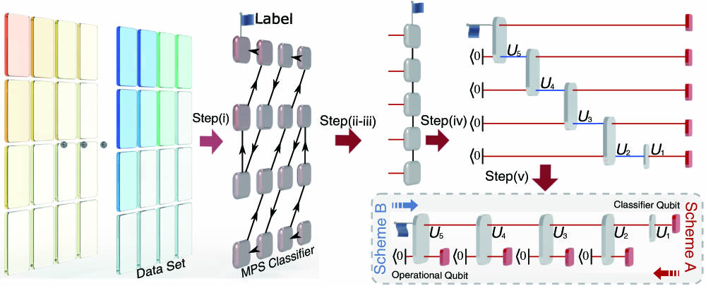
Figure 1.Illustration of the main steps of implementing the TN-based quantum classifier. In steps (i)–(iii), we map the images of $N = 784$ pixels (features) to quantum states and train the matrix product state (MPS) classifier using these images in the MNIST dataset by a supervised learning algorithm. The MPS consists of $N$ tensors represented by squares, with the label index represented by a flag. We calculate the entanglement entropies of the MPS and retain only $\tilde{N} = 3$ or 5 features with the largest entanglement entropies. Then, we train a reduced MPS with the $\tilde{N}$ retained features. In steps (iv) and (v), the reduced MPS is translated to a circuit acting on $\tilde{N}$ qubits and further to a circuit using the qubit-efficient scheme, which involves ${\tilde{N}}^{'} = 2$ qubits and $\tilde{N}$ gates, including a single-qubit gate $U_{1}$ and $\tilde{N} - 1$ two-qubit gates $U_{i}$ ( $i = 2, 3$ or $i = 2, \dots, 5$ ). We employ two schemes to implement the classifier, whose orders of operations are indicated by the red and blue arrows, respectively.

In Fig. 2, with increasing $\tilde{N}$ , the testing accuracy and training accuracy for the MNIST dataset both increase quickly as expected. More importantly, both accuracies converge for $\tilde{N} \geq 10$ . For $\tilde{N} = 3 o r 5$ , both accuracies are higher than 0.98, which implies that the reduced number of the feature qubits works well for the TN-based quantum classifier.

Figure 2.Training and testing accuracies of classifying the “0” and “1” digits in the MNIST dataset as functions of $\tilde{N}$ . Data are obtained by averaging the accuracies over 20 numerical simulations, and error bars indicate the statistical uncertainty.

The subsequent experimental implementation involves the following two steps (see Appendix B for more details). In step (iv), we translate the tensors in the optimized MPS to a quantum circuit, which form a circuit acting on $\tilde{N}$ qubits [42]. In step (v), through the quantum-efficient scheme [26], the quantum circuit is further simplified to the one with $\tilde{N}$ gates acting on ${\tilde{N}}^{'}$ qubits. We take ${\tilde{N}}^{'} = 2$ , where two qubits are dubbed as the operational and classifier qubits. This is achieved by translating measurements on different qubits into those on only two qubits at different times. The extracted features of an image are input to the circuit by measuring the operational qubit at different times. The output of the image classifier is accessed via projective measurements on the classifier qubit.

We present two schemes of TN-based quantum classifiers, each being the reverse of the other. In either case, we embed core features of an image into the quantum feature space of three or five feature states ${| ψ_{i} ⟩}$ , which corresponds to a three- or five-layer construction that involves their respective number of unitary gate operations.

In Scheme A, we initialize the classifier and operational qubits into feature states $| ψ_{1} ⟩$ and $| ψ_{2} ⟩$ , respectively. Other feature states $| ψ_{i} ⟩$ are used as successive inputs for the optimized quantum circuit consisting of a series of single- and two-qubit gates $U_{i}$ . Taking the three-layer construction as an example, the classifier qubit is subject to the single-qubit operator $U_{1}$ , whose output is fed into the two-qubit operation $U_{2}$ together with the operational qubit. After projecting the operational qubit into the basis state $| 0 ⟩$ , the classifier qubit is characterized by the density matrix, $ρ_{1} = {Tr}_{op} [U_{2} (U_{1} | ψ_{1} ⟩ ⟨ ψ_{1} | U_{1}^{†} \otimes | ψ_{2} ⟩ ⟨ ψ_{2} |) U_{2}^{†} (1 \otimes | 0 ⟩ ⟨ 0 |)] .$ Here, ${Tr}_{op}$ is the trace over the two-dimensional Hilbert space of the operational qubit. The operational qubit is then prepared in the feature state $| ψ_{3} ⟩$ , before the two-qubit operator $U_{3}$ is applied on both qubits. After projecting the operational qubit into the basis state $| 0 ⟩$ again, the classifier qubit is given by $ρ_{2} = {Tr}_{op} [U_{3} (ρ_{1} \otimes | ψ_{3} ⟩ ⟨ ψ_{3} |) U_{3}^{†} (1 \otimes | 0 ⟩ ⟨ 0 |)] .$

We perform a projective measurement of $σ_{z} = | 0 ⟩ ⟨ 0 | - | 1 ⟩ ⟨ 1 |$ on the output classifier qubit, yielding probabilities $P_{0}$ and $P_{1}$ . The image is recognized as “0” (“1”) for $P_{0} > P_{1}$ ( $P_{1} > P_{0}$ ).

In Scheme B, we initialize the classifier and operational qubits into the two-qubit state $| 00 ⟩$ (or $| 10 ⟩$ ), and successively apply the optimized unitary gates $U_{i}^{†}$ (in the reverse order compared to that in Scheme A). A projective measurement $| ψ_{i} ⟩ ⟨ ψ_{i} |$ is performed following the corresponding unitary operation $U_{i}^{†}$ . The last projective measurement $| ψ_{1} ⟩ ⟨ ψ_{1} |$ on the classifier qubit yields the probability $P_{0}^{'}$ ( $P_{1}^{'}$ ) for the initial state $| 00 ⟩$ (or $| 10 ⟩$ ). Since $P_{0} = P_{0}^{'}$ and $P_{1} = P_{1}^{'}$ (see the derivations in Appendix C), the image is recognized as “0” (“1”) for $P_{0}^{'} > P_{1}^{'}$ ( $P_{1}^{'} > P_{0}^{'}$ ).

3. EXPERIMENTAL REALIZATION

Experimentally, we encode the classifier qubit in the polarization states of the signal photons, i.e., $| H ⟩ = | 0 ⟩$ and $| V ⟩ = | 1 ⟩$ (see Fig. 3). The operational qubit is encoded in the spatial modes of the photons, with $| u ⟩ = | 0 ⟩$ and $| d ⟩ = | 1 ⟩$ representing the upper and lower spatial modes, respectively. While the single-qubit gate $U_{1}$ is implemented using a half-wave plate (HWP), the two-qubit gates $U_{i}$ ( $i = 2, 3$ ) are implemented through cascaded interferometers, consisting of HWPs and beam displacers (BDs). In Scheme A, feature states $| ψ_{i} ⟩$ ( $i = 2, 3$ ) are introduced via a controlled beam splitter (CBS), which consists of HWPs and BDs, with information of the feature states encoded in the setting angles of the HWPs.

Figure 3.Experimental demonstration of quantum classifier with the three-layer construction. For each pair of photons generated by spontaneous parametric down conversion, one photon serves as the trigger, and the other, the signal photon, proceeds through the experimental setup corresponding to the two schemes. Under Scheme A, the signal photon is projected onto the polarization state $| ψ_{1} ⟩$ of the classifier qubit via a PBS and an HWP $H_{0}$ . It is then sent through an interferometric network, composed of HWPs and BDs, before being detected by APDs in coincidence with the trigger photon. The single-qubit gate $U_{1}$ is realized by an HWP, and two-qubit gates $U_{2}$ and $U_{3}$ are realized by BDs and HWPs. The input states $| ψ_{2} ⟩$ and $| ψ_{3} ⟩$ are encoded in the spatial modes of photons and prepared via the HWPs ( $H_{1}$ , $H_{2}$ , $H_{9}$ , and $H_{10}$ ) in controlled beam splitters (CBSs), which, by combining the spatial and polarization degrees of freedom, effectively expand the dimension of the system. A 1 m long single-mode fiber serves as a spatial filter in between successive modules of the two-qubit gate, and a set of wave plates is introduced to offset the impact of the fiber on the photon polarizations. For detection, photons are projected onto the upper spatial mode $| u ⟩$ by discarding those in the lower one, and a projective measurement of $σ_{z}$ is realized through an HWP, a PBS, and APDs. Scheme B is the exact reverse process of Scheme A, where photons are sent into the setup through the output port of Scheme A.

The gates are trained by 12,665 hand-written digits of “0” and “1” in the training set of the MNIST dataset [27]. After the training process, $U_{i}$ are fixed for subsequent image recognition. To assess the training process, we first use 2115 images in the testing set of the MNIST dataset as input. Specifically, we use all the training images of “0” and “1” for training and all testing images for testing in the MNIST dataset, which are all downloaded from the official website. As illustrated in Fig. 4, under the three-layer construction, the classifier fails to recognize only 30 out of the 2115 images, including 10 images of “0” and 20 images of “1”. The success probability of classification is 0.9858. Under the five-layer construction, the classifier fails to recognize 19 images within the same testing set, including four images of “0” and 15 images of “1”. The success probability is 0.9910.

Figure 4.Theoretical results of the testing set under the (a) three- and (b) five-layer constructions, respectively. The output states are shown in the $x − z$ plane of the Bloch sphere associated with the classifier qubit. The green squares (blue triangles) indicate successful recognition of the hand-written digit “0” (“1”). Red symbols indicate cases in which the classifier fails to recognize the image.

Figure 5 demonstrates in detail the results of several typical testing images as examples. For all chosen images, the experimental results suggest that the classifiers are well-trained, in the sense that their predictions have a high success rate, even if the probability difference $P_{0} - P_{1}$ ( $P_{0}^{'} - P_{1}^{'}$ ) can be small for certain cases. Furthermore, some images that cannot be classified under the three-layer construction can be successfully classified under the five-layer construction, confirming the improvement in behavior of the quantum classifier with an increased feature-space dimension.

Figure 5.Experimental classification of images within the testing set. Measured probabilities of the projective measurements on output states of quantum classifiers with the (a) three- and (b) five-layer constructions. Left, Scheme A; right, Scheme B. Colored bars represent experimental results, while hollow bars represent their theoretical predictions. Error bars indicate the statistical uncertainty, obtained by assuming Poissonian statistics in the photon-number fluctuations. (c) The classification results for eight typical hand-written digits in the testing set. Rows represent the index of images, namely the hand-written digits, the experimental and theoretical probability differences, and classification results. $P_{0,1}^{3}$ and $P_{0,1}^{5}$ represent probabilities associated with the three- and five-layer constructions, respectively.

To estimate the deviation of the experimental results and theoretical predictions, we define a distance, $d := \sqrt{\frac{{(P_{0} - P_{0}^{th})}^{2} + {(P_{1} - P_{1}^{th})}^{2}}{2}},$ where $P_{0,1}$ and $P_{0,1}^{th}$ are the measured probabilities and theoretical probabilities, respectively. The distance varies between 0 and 1, with 0 indicating a perfect match. Of all eight distances for the images in Fig. 5, the largest is $0.039 \pm 0.003$ , which indicates that our experimental results are in excellent agreement with theoretical predictions.

The differences between the experimental data and theoretical predictions are caused by several factors, including fluctuations in photon numbers, the inaccuracy of wave plates, and the dephasing due to the misalignment of the BDs. To provide a quantitative estimate of the success rate of our quantum classifier, we perform numerical simulations by taking experimental imperfections into account.

First, the imperfection caused by photon-number fluctuations increases with decreasing photon counts. In our experiment, the total photon count for each image classification is larger than $10^{4}$ . Therefore, we adopt a total photon count of $10^{4}$ for our estimation, while assuming a Poissonian distribution in the photon statistics. Second, parameters characterizing the inaccuracy of wave plates and the dephasing are estimated using experimental data in Fig. 5. Specifically, for each wave plate, we assume an uncertainty in the setting angle $θ + δ θ$ , where $δ θ$ is randomly chosen from the interval $[- 1.588 °, 1.588 °]$ ( $[- 1.180 °, 1.180 °]$ ) under the three-layer (five-layer) construction. The range of these intervals is determined through Monte Carlo simulations to fit the deviations of experimental data from their theoretical predictions for the eight images in Fig. 5. On the other hand, the dephasing due to the misalignment of BDs affects the experimental results through a noisy channel $ε (ρ) = η ρ + (1 - η) σ_{z} ρ σ_{z}$ characterized by a dephasing rate $η$ [43], where $ρ$ [ $ε (ρ)$ ] is the density matrix of the input (output) state of the noisy channel. By numerically minimizing the difference between the numerical results and the corresponding experiment data, we estimate $η$ to be 0.9977 (0.9926) for three-layer (five-layer) construction.

With these, we perform Monte Carlo simulations of our experiments on all 2115 images in the testing set, from which a success rate is estimated. We then repeat the process 100 times and keep the lowest success rate as our final estimation. The estimated success rates are the following: 0.9825 (Scheme A with three-layer construction); 0.9820 (Scheme B with three-layer construction); 0.9877 (Scheme A with five-layer construction); 0.9877 (Scheme B with five-layer construction). Thus, for all experiments, the success rates are above 98%.

In Fig. 6, we show the results of applying the trained classifier on two pairs of hand-written digits “0” and “1” that are not in the MNIST dataset. The first pair of digits is written in a standard way. The second pair is written such that the profile of “0” resembles that of “1” in the first pair, and the profile of “1” is much shorter and fatter compared to its counterpart in the first pair. For both cases, our classifier correctly recognizes the images with high confidence (large $| P_{0} - P_{1} |$ ), demonstrating the robustness and accuracy of the device.

Figure 6.Classification of images outside the MNIST dataset. (a) Measured probabilities of the output states of quantum classifiers. (b) Classification results.

4. DISCUSSION

We report the first, to the best of our knowledge, experimental demonstration of quantum binary classification of real-life, hand-drawn images with single photons. The experimental scheme adopts a TN-based ML algorithm, which benefits from the powerful interpretability of TNs, as well as the efficient entanglement-based optimization in the quantum feature space. After training and optimizing the classifier on classical computers, we use single photons to achieve the binary classification with a success rate over 98%. Our experiment can be readily extended to multi-category classification by taking advantage of the multiple degrees of freedom of photons and specially designed interferometric network for single- and two-qubit operations. The hybrid quantum-classical scheme demonstrated here can be upgraded to be fully quantum mechanical, if the optimization in the ML process is performed on device parameters (such as the setting angles of wave plates), rather on the overall design of quantum circuits. Furthermore, the TN-based ML algorithm is general and directly applicable to a wide range of physical systems that have full control of qubits/qudits, including nitrogen-vacancy centers [39], nuclear magnetic resonance systems [12], and trapped ions [29]. In particular, with the rapid progress in quantum computers based on superconducting quantum circuits [30], it is hopeful that TN-based ML can be demonstrated for a larger feature space with more qubits, such that it can find utilities in more complicated real-world tasks.

Acknowledgment

Acknowledgment. We thank Barry C. Sanders for providing constructive criticism on the paper.

APPENDIX A: TENSOR-NETWORK MACHINE LEARNING ALGORITHM

N

N_{c}

| Ψ ⟩ = \sum_{{s}} \sum_{{a}} \sum_{c} A_{s_{N}, c a_{N - 1}}^{[N]} \dots A_{s_{2}, a_{2} a_{1}}^{[2]} A_{s_{1}, a_{1}}^{[1]} \otimes_{n = 1}^{N} | i_{n} ⟩ | c ⟩ .

\dim (c) = N_{c} = 2

f = - \sum_{m \in I} \ln P_{c^{(m)}},

A^{[i]}

{| ψ_{i} ⟩}

| s_{n} ⟩

N

H

To complete the feature extraction of the image, we retain a small number of feature qubits (three or five feature qubits corresponding to three- or five-layer constructions) that have the largest entanglement entropy in the quantum feature space, according to Eq. (A9) [25], to represent and classify hand-written digits of “0” and “1” in the MNIST dataset. It is crucial for implementing the classifier on our photonic simulator under three- or five-layer constructions, respectively. We note that since high-frequency components of the original image are mostly discarded in the cosine transformation, our scheme should also be robust to high-frequency noise in the hand-drawn image.

In our practical simulations of the “0” and “1” MPS classifier, the tensors in the MPS are initialized randomly. In consideration of efficiency, we randomly take 2000 images from the training set to train the MPS. The testing accuracy is evaluated by all the “0” and “1” digits in the testing set. The results can be reproduced by the code from Ref. [46].

APPENDIX B: QUBIT-EFFICIENT QUANTUM CIRCUITS

\tilde{N}

⟨ 0 c | U_{N} U_{N}^{†} | 1 c^{'} ⟩ = 0,

After getting the matrix elements of all gate operations, we numerically determine the parameters of the photonic interferometry network.

The circuit still requires as many qubits as the retained features. To further reduce the number of qubits to two, we adopt the quantum-efficient scheme [26] [step (v)], which is achieved by translating measurements on different qubits into those on only two qubits (the operational and classifier qubits) at different times. The extracted features of an image are input to the circuit by measuring the operational qubit at different times, while the information is carried by the classifier qubit, which can be extracted using projective measurements.

APPENDIX C: EQUIVALENCE BETWEEN TWO SCHEMES OF QUANTUM CLASSIFIERS

| 00 ⟩

Figure 7.Experimental demonstration of quantum classifier under Scheme B (three-layer construction). The classifier and operational qubits are initialized in $| H ⟩ \otimes | u ⟩$ or $| V ⟩ \otimes | u ⟩$ via a PBS and an HWP. After each gate operation $U_{i}^{†}$ ( $i = 1, 2, 3$ ), a projective measurement $| ψ_{i} ⟩ ⟨ ψ_{i} |$ is performed on the operational qubit via a CBS. This is the reverse process of the setup in Fig. 1 of the main text.

σ_{z}

P_{0} + P_{1} = P_{0}^{'} + P_{1}^{'} = 1

APPENDIX D: EXPERIMENTAL DETAILS

| H ⟩

2 \times 10^{4}

U_{1}

U_{i}

References

[1] J. Biamonte, P. Wittek, N. Pancotti, P. Rebentrost, N. Wiebe, S. Lloyd. Quantum machine learning. Nature, 549, 195-202(2017).

[2] V. Dunjko, H. J. Briegel. Machine learning & artificial intelligence in the quantum domain: a review of recent progress. Rep. Prog. Phys., 81, 074001(2018).

[3] V. Havlíčeka, A. D. Córcoles, K. Temme, A. W. Harrow, A. Kandala, J. M. Chow, J. M. Gambetta. Supervised learning with quantum-enhanced feature spaces. Nature, 567, 209-212(2019).

[4] I. Cong, S. Choi, M. D. Lukin. Quantum convolutional neural networks. Nat. Phys., 15, 1273-1278(2019).

[5] M. Schuld, N. Killoran. Quantum machine learning in feature Hilbert spaces. Phys. Rev. Lett., 122, 040504(2019).

[6] F. Verstraete, V. Murg, J. I. Cirac. Matrix product states, projected entangled pair states, and variational renormalization group methods for quantum spin systems. Adv. Phys., 57, 143-224(2008).

[7] J. I. Cirac, F. Verstraete. Renormalization and tensor product states in spin chains and lattices. J. Phys. A, 42, 504004(2009).

[8] J. Haegeman, F. Verstraete. Diagonalizing transfer matrices and matrix product operators: a medley of exact and computational methods. Annu. Rev. Condens. Matter Phys., 8, 355-406(2017).

[9] S.-J. Ran, E. Tirrito, C. Peng, X. Chen, L. Tagliacozzo, G. Su, M. Lewenstein. Tensor Network Contractions(2020).

[10] Z.-Z. Sun, C. Peng, D. Liu, S.-J. Ran, G. Su. Generative tensor network classification model for supervised machine learning. Phys. Rev. B, 101, 075135(2020).

[11] P. Rebentrost, M. Mohseni, S. Lloyd. Quantum support vector machine for big data classification. Phys. Rev. Lett., 113, 130503(2014).

[12] Z. Li, X. Liu, N. Xu, J. Du. Experimental realization of a quantum support vector machine. Phys. Rev. Lett., 114, 140504(2015).

[13] D. Anguita, S. Ridella, F. Rivieccio, R. Zunino. Quantum optimization for training support vector machines. Neural Netw., 16, 763-770(2003).

[14] Y.-Z. You, Z. Yang, X.-L. Qi. Machine learning spatial geometry from entanglement features. Phys. Rev. B, 97, 045153(2018).

[15] Y. Levine, O. Sharir, N. Cohen, A. Shashua. Quantum entanglement in deep learning architectures. Phys. Rev. Lett., 122, 065301(2019).

[16] D.-L. Deng, X. Li, S. Das Sarma. Quantum entanglement in neural network states. Phys. Rev. X, 7, 021021(2017).

[17] D. D. Lee, E. Stoudenmire, M. Sugiyama, D. J. Schwab, U. V. Luxburg, I. Guyon, R. Garnett. Supervised learning with tensor networks. Advances in Neural Information Processing Systems, 29, 4799-4807(2016).

[18] D. Liu, S.-J. Ran, P. Wittek, C. Peng, R. B. Garca, G. Su, M. Lewenstein. Machine learning by unitary tensor network of hierarchical tree structure. New J. Phys., 21, 073059(2019).

[19] Z.-Y. Han, J. Wang, H. Fan, L. Wang, P. Zhang. Unsupervised generative modeling using matrix product states. Phys. Rev. X, 8, 031012(2018).

[20] C. Guo, Z. Jie, W. Lu, D. Poletti. Matrix product operators for sequence-to-sequence learning. Phys. Rev. E, 98, 042114(2018).

[21] E. M. Stoudenmire. Learning relevant features of data with multi-scale tensor networks. Quantum Sci. Technol., 3, 034003(2018).

[22] S. Cheng, L. Wang, T. Xiang, P. Zhang. Tree tensor networks for generative modeling. Phys. Rev. B, 99, 155131(2019).

[23] I. Glasser, R. Sweke, N. Pancotti, J. Eisert, I. J. Cirac. Expressive power of tensor-network factorizations for probabilistic modeling. Advances in Neural Information Processing Systems, 32, 1496-1508(2019).

[24] S. Efthymiou, J. Hidary, S. Leichenauer. TensorNetwork for machine learning(2019).

[25] Y. Liu, X. Zhang, M. Lewenstein, S.-J. Ran. Entanglement-guided architectures of machine learning by quantum tensor network(2018).

[26] W. Huggins, P. Patil, B. Mitchell, K. B. Whaley, E. M. Stoudenmire. Towards quantum machine learning with tensor networks. Quantum Sci. Technol., 4, 024001(2019).

[27] L. Deng. The MNIST database of handwritten digit images for machine learning research [best of the web]. IEEE Signal Process. Mag., 29, 141-142(2012).

[28] X.-D. Cai, D. Wu, Z.-E. Su, M.-C. Chen, X.-L. Wang, L. Li, N.-L. Liu, C.-Y. Lu, J.-W. Pan. Entanglement-based machine learning on a quantum computer. Phys. Rev. Lett., 114, 110504(2015).

[29] D.-B. Zhang, S.-L. Zhu, Z. D. Wang. Protocol for implementing quantum nonparametric learning with trapped ions. Phys. Rev. Lett., 124, 010506(2020).

[30] F. Arute, K. Arya, R. Babbush, D. Bacon, J. C. Bardin, R. Barends, R. Biswas, S. Boixo, F. G. S. L. Brandao, D. A. Buell, B. Burkett, Y. Chen, Z. Chen, B. Chiaro, R. Collins, W. Courtney, A. Dunsworth, E. Farhi, B. Foxen, A. Fowler, C. Gidney, M. Giustina, R. Graff, K. Guerin, S. Habegger, M. P. Harrigan, M. J. Hartmann, A. Ho, M. Hoffmann, T. Huang, T. S. Humble, S. V. Isakov, E. Jeffrey, Z. Jiang, D. Kafri, K. Kechedzhi, J. Kelly, P. V. Klimov, S. Knysh, A. Korotkov, F. Kostritsa, D. Landhuis, M. Lindmark, E. Lucero, D. Lyakh, S. Mandrà, J. R. McClean, M. McEwen, A. Megrant, X. Mi, K. Michielsen, M. Mohseni, J. Mutus, O. Naaman, M. Neeley, C. Neill, M. Y. Niu, E. Ostby, A. Petukhov, J. C. Platt, C. Quintana, E. G. Rieffel, P. Roushan, N. C. Rubin, D. Sank, K. J. Satzinger, V. Smelyanskiy, K. J. Sung, M. D. Trevithick, A. Vainsencher, B. Villalonga, T. White, Z. J. Yao, P. Yeh, A. Zalcman, H. Neven, J. M. Martinis. Quantum supremacy using a programmable superconducting processor. Nature, 574, 505-510(2019).

[31] A. Pepper, N. Tischler, G. J. Pryde. Experimental realization of a quantum autoencoder: the compression of qutrits via machine learning. Phys. Rev. Lett., 122, 060501(2019).

[32] H.-K. Lau, R. Pooser, G. Siopsis, C. Weedbrook. Quantum machine learning over infinite dimensions. Phys. Rev. Lett., 118, 080501(2017).

[33] X. Gao, Z.-Y. Zhang, L.-M. Duan. A quantum machine learning algorithm based on generative models. Sci. Adv., 4, eaat9004(2018).

[34] D. Zhu, N. M. Linke, M. Benedetti, K. A. Landsman, N. H. Nguyen, C. H. Alderete, A. Perdomo-Ortiz, N. Korda, A. Garfoot, C. Brecque, L. Egan, O. Perdomo, C. Monroe. Training of quantum circuits on a hybrid quantum computer. Sci. Adv., 5, eaaw9918(2019).

[35] K. Bartkiewicz, C. Gneiting, A. Černoch, K. Jiráková, K. Lemr, F. Nori. Experimental kernel-based quantum machine learning in finite feature space. Sci. Rep., 10, 12356(2020).

[36] J. Gao, L.-F. Qiao, Z.-Q. Jiao, Y.-C. Ma, C.-Q. Hu, R.-J. Ren, A.-L. Yang, H. Tang, M.-H. Yung, X.-M. Jin. Experimental machine learning of quantum states. Phys. Rev. Lett., 120, 240501(2018).

[37] L. Hu, S.-H. Wu, W. Cai, Y. Ma, X. Mu, Y. Xu, H. Wang, Y. Song, D.-L. Deng, C.-L. Zou, L. Sun. Quantum generative adversarial learning in a superconducting quantum circuit. Sci. Adv., 5, eaav2761(2019).

[38] A. Hentschel, B. C. Sanders. Machine learning for precise quantum measurement. Phys. Rev. Lett., 104, 063603(2010).

[39] W. Lian, S.-T. Wang, S. Lu, Y. Huang, F. Wang, X. Yuan, W. Zhang, X. Ouyang, X. Wang, X. Huang, L. He, X. Chang, D.-L. Deng, L. Duan. Machine learning topological phases with a solid-state quantum simulator. Phys. Rev. Lett., 122, 210503(2019).

[40] P. Xue, Y.-F. Xiao. Universal quantum computation in decoherence-free subspace with neutral atoms. Phys. Rev. Lett., 97, 140501(2006).

[41] P. Xue, B. C. Sanders, D. Leibfried. Quantum walk on a line for a trapped ion. Phys. Rev. Lett., 103, 183602(2009).

[42] C. Schön, E. Solano, F. Verstraete, J. I. Cirac, M. M. Wolf. Sequential generation of entangled multiqubit states. Phys. Rev. Lett., 95, 110503(2005).

[43] K. Wang, X. Wang, X. Zhan, Z. Bian, J. Li, B. C. Sanders, P. Xue. Entanglement-enhanced quantum metrology in a noisy environment. Phys. Rev. A, 97, 042112(2018).

[44] D. Pérez-García, F. Verstraete, M. M. Wolf, J. I. Cirac. Matrix product state representations. Quantum Inf. Comput., 7, 401-430(2007).

[45] C. M. Bishop. Pattern Recognition and Machine Learning(2006).

[46] https://github.com/YuhanLiuSYSU/MPS_ImageClassifier. https://github.com/YuhanLiuSYSU/MPS_ImageClassifier

[47] L. Xiao, X. Zhan, Z.-H. Bian, K. Wang, X. Zhang, X.-P. Wang, J. Li, K. Mochizuki, D. Kim, N. Kawakami, W. Yi, H. Obuse, B. C. Sanders, P. Xue. Observation of topological edge states in parity–time-symmetric quantum walks. Nat. Phys., 13, 1117-1123(2017).

[48] J. A. Izaac, X. Zhan, Z. Bian, K. Wang, J. Li, J. Wang, P. Xue. Centrality measure based on continuous-time quantum walks and experimental realization. Phys. Rev. A, 95, 032318(2017).