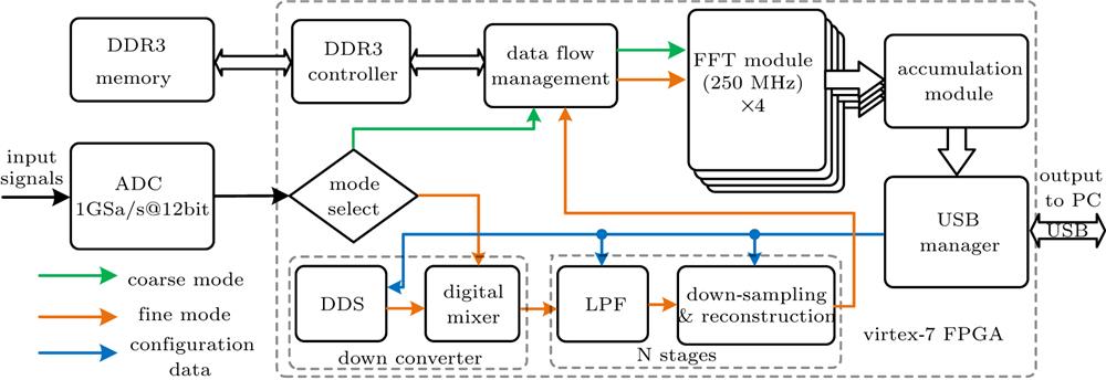
Fig. 1. The architecture of the high performance FFT spectrum analyzer. Two optional operating modes are designed using the reconfigurable FPGA resources.

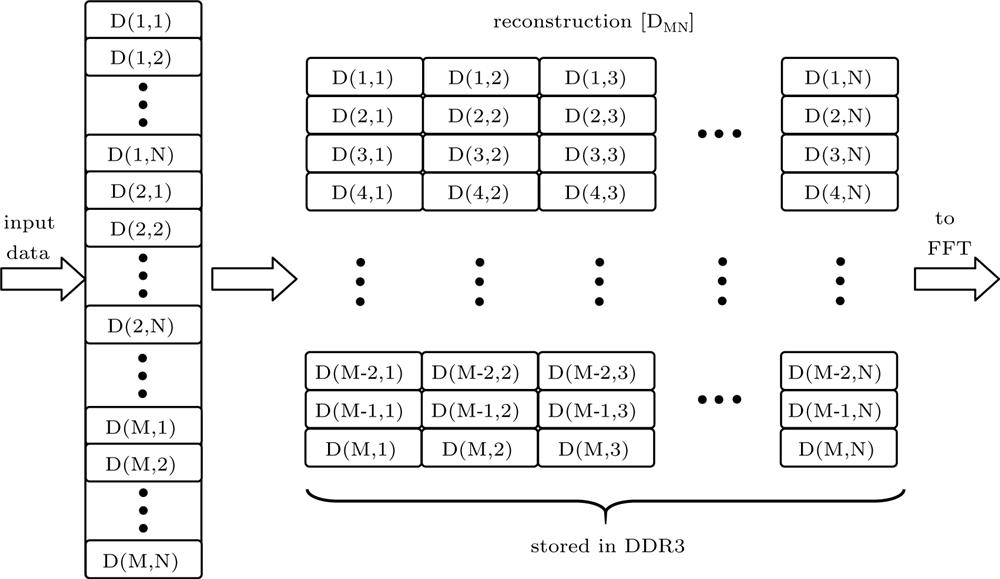
Fig. 2. The block diagram of the down-sampling and reconstruction module. The input data are reconstructed by using N stages of data down-sampling and reconstruction, and the digital data after reconstruction are processed by the FFT module.

Fig. 3. The frequency spectrums before and after down-sampling and filtering. (a)–(c) The produced signal aliasing when performing down-sampling. (d)–(f) The signal aliasing suppressed effectively by the implementation of the multi-stage filters.

Fig. 4. Block diagram of customized software for the FFT spectrum analyzer.

Fig. 5. Spin noise measurements for alkali metal Rb. (a)–(c) FFT spectrums measured with coarse mode, data reconstruction, and fine mode, respectively. In the fine mode, the input data are processed successively by the down converting module, the multi-stage digital filters, the multi-stage data reconstruction module, and the FFT module.

Fig. 6. The plots of the signal-to-noise-ratio versus the time span of spin noise measurements: (a) and (b) with a 1/4 GSa/s sampling rate, (c) and (d) with a 1/16 GSa/s sampling rate, (e) and (f) with a 1/256 GSa/s sampling rate.

Fig. 7. The test results of measuring mixed signals with different frequency components. Utilizing the high performance FFT spectrum analyzer to obtain the FFT spectrums, the mixed signals can be measured with a high frequency resolution, and the signals aliasing can be suppressed.

Fig. 8. The plots of frequency response characteristics of the filter. (a), (b) The filters operating at a 1/256 GSa/s and a 1 GSa/s sampling rates, respectively.

Table 1. Efficiency comparison between this work and the software based FFT.

Table 2. Resource occupation of the hardware accelerated FFT DAQ board.

Table 3. Performance comparison among FFT DAQs.