Human Pose Estimation Based on Secondary Generation Adversary

Xiankun Zhang; Rongfen Zhang; Yuhong Liu

doi:10.3788/LOP57.201509

Journals >Laser & Optoelectronics Progress >Volume 57 >Issue 20 >Page 201509 > Article

Laser & Optoelectronics Progress
Vol. 57, Issue 20, 201509 (2020)

Human Pose Estimation Based on Secondary Generation Adversary

Xiankun Zhang, Rongfen Zhang, and Yuhong Liu^*

Author Affiliations

Key Laboratory of Big Data and Intelligent Technology, College of Big Data and Information Engineering, Guizhou University, Guiyang, Guizhou 550025, China

show less

DOI: 10.3788/LOP57.201509 Cite this Article Set citation alerts

Xiankun Zhang, Rongfen Zhang, Yuhong Liu. Human Pose Estimation Based on Secondary Generation Adversary[J]. Laser & Optoelectronics Progress, 2020, 57(20): 201509 Copy Citation Text

show less

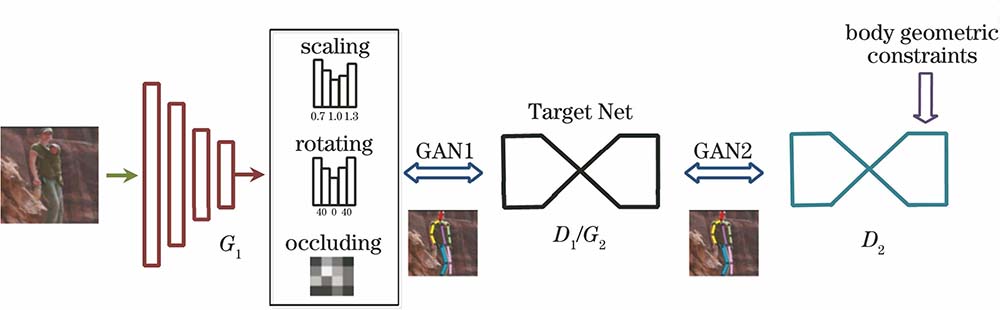
Fig. 1. Structure schematic diagram of our method

Download full size

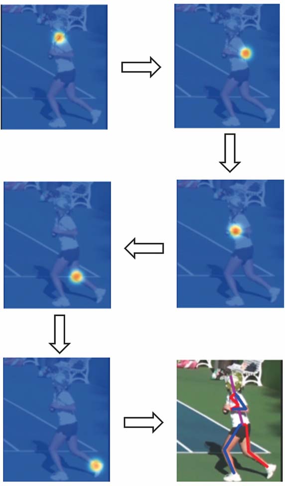
Fig. 2. Schematic diagram of heatmap

Download full size

Fig. 3. Structure of hourglass network

Download full size

Fig. 4. Cascade structure diagram of SHN

Download full size

Fig. 5. Structure of intermediate supervision

Download full size

Fig. 6. Procedure of ASR

Download full size

Fig. 7. Procedure of AHO

Download full size

Fig. 8. Reconstruction of heatmap

Download full size

Fig. 9. Heatmaps obtained by different methods. (a) Ref. [4]; (b) Ref. [10]; (c) Ref. [11]; (d) ours

Download full size

Fig. 10. Comparison of joint estimation errors

Download full size

Input: a mini-batch training image set X
1.X is randomly and equally divided into X₁、X₂、X₃;2.Train D₁ using X₁;3.Train G₁、D₁ using X₂ with table 2 on ASR;4.Train G₁、D₁ using X₃ with table 2 on AHO.

Table 1. Training process of batch images

Input: image x

1.Get shortcut features from D₁;2.Get distribution P from shortcut features in G₁;3.Sample an adversarial augmentation data

\overset{︵}{x}

from P;4.Compute the loss of D₁:

{\overset{︵}{L}}_{MSE}

with

\overset{︵}{x}

;5.Random augment x to get

\overset{︵}{x}

;6.Compute the loss of D₁:

{\overset{︵}{L}}_{MSE}

with

\overset{︵}{x}

;7.Compare

\overset{︵}{L}

and

\overset{︵}{L}

with formula (5) and formula (6) to update G₁;8.Update D₁.

Table 2. Training process of single image

Input: image x;ground truth heatmap C
1. D₂ reconstructs heatmap: D(C,x);2. Compute L_real with formula (11);3. G₂ generates predictive heatmap: $\tilde{C}$ =G(x);4. Compute L_MSE with formula (8);5. D₂ reconstructs heatmap:D( $\tilde{C}$ ,x);6. Compute $p_{\tilde{C}}$ ;7. Compute L_fake、L '_D with formula (11)、formula (12);8. Update D₂;9. Compute L_adv、L_G with formula (9)、formula (10);10.Update G₂.

Table 3. Training process of the secondary generation adversary

Method	Head	Shoulder	Elbow	Wrist	Hip	Knee	Ankle	Mean
Ref. [21]	97.8	92.5	87.0	83.9	91.5	90.8	89.9	90.5
Ref. [4]	98.2	94.0	91.2	87.2	93.5	94.5	92.6	93.0
Ref. [12]	98.5	94.0	89.8	87.5	93.9	94.1	93.0	93.1
Ref. [10]	98.6	95.3	92.8	90.0	94.8	95.3	94.5	94.5
Ref. [11]	98.2	94.9	92.2	89.5	94.2	95.0	94.1	94.0
Ours	98.8	95.7	92.6	90.8	94.8	96.1	95.0	94.8

Table 4. PCK of different methods in LSP data setunit: %

Method	Head	Shoulder	Elbow	Wrist	Hip	Knee	Ankle	Mean
Ref. [21]	97.8	95.0	88.7	84.0	88.4	82.8	79.4	88.5
Ref. [4]	98.2	96.3	91.2	87.1	90.1	87.4	83.6	90.9
Ref. [12]	98.6	96.2	90.9	86.7	89.8	87.0	83.2	90.6
Ref. [10]	98.1	96.6	92.5	88.4	90.7	87.7	83.5	91.5
Ref. [11]	98.2	96.8	92.2	88.0	91.3	89.1	84.9	91.8
Ours	98.4	97.1	93.4	88.7	92.5	90.3	85.2	92.2

Table 5. PCKh of different methods in the MPII data setunit: %

Method	Convergenceiteration times	Average processingtime /s	GFLOPs /(10⁹ times)	Number ofparameters /10⁷
Ref. [11]	19500	0.48	10.820	5.495
Ours	26600	0.73	13.702	6.738

Table 6. Comparison of model efficiency

Xiankun Zhang, Rongfen Zhang, Yuhong Liu. Human Pose Estimation Based on Secondary Generation Adversary[J]. Laser & Optoelectronics Progress, 2020, 57(20): 201509

Download Citation

Set citation alerts for the article

Tools

Set citation alerts for the article

Save the article for my favorites

Paper Information