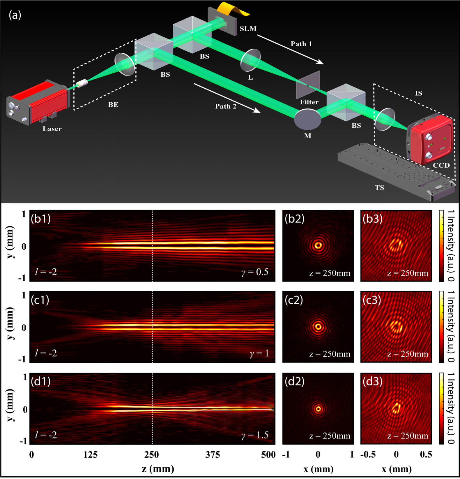
Fig. 1. Experimental observations of POVBs in free space for different values of the phase modulation exponent γ. (a) Schematic of the experimental setup used for the generation and detection of the POVBs. Path 1 highlights the beamline used for the generation, while path 2 the beamline used for carrying out the interferograms. (b1)–(d1) Normalized side-view of the beams in the y−z plane for (b1) γ=0.5, (c1) γ=1, and (d1) γ=1.5. (b2)–(d2) Intensity distributions and (b3)–(d3) interferograms recorded at the distance z=250  mm, marked by dashed white lines in (b1)–(d1). l=−2 is the topological charge. L, lens; M, mirror; BE, beam expander; BS, beam splitter; IS, imaging system; TS, translation stage; SLM, spatial light modulator.

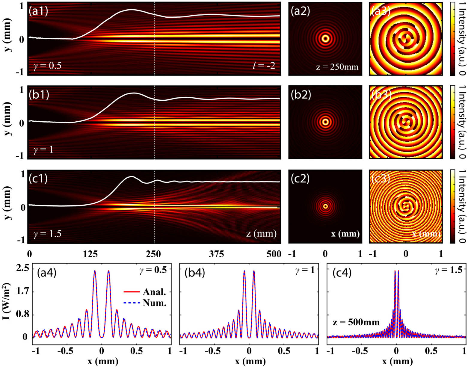
Fig. 2. Numerical simulation of POVBs for different values of the parameter γ, with topological charge l=−2 and initial amplitudes predesigned to achieve a low-varying peak intensity over a long range of distances. (a1)–(c1) Normalized longitudinal intensity distributions in the y−z plane for (a1) γ=0.5, (b1) 1, and (c1) 1.5; solid white lines in each panel plot the peak intensity evolutions. Corresponding (a2)–(c2) transverse intensity distributions and (a3)–(c3) wrapped phase patterns extracted at a distance z=250  mm, marked by dashed white lines in (a1)–(c3). (a4)–(c4) Comparison between numerical (blue dashed lines) intensity profiles in (a1)–(c1) and analytical (red solid lines) prediction from Eq. (3), performed at the output after 500 mm long propagation.

Fig. 3. Numerical (left) and experimental (right) results of POVBs in free space with γ=1.5, topological charge l=−2, and different initial amplitudes designed to achieve a desired peak intensity evolution. Left-column panels illustrate the normalized longitudinal intensity distributions of POVBs whose peak intensity along the propagation direction follows (a1) a hyperbolic secant, (b1) a flat-top, and (c1) a sinusoidal curve as marked by a solid white line in each panel. Right-column panels show the corresponding experimental results. To provide a better comparison, experimental peak intensity evolutions (yellow dots) extracted from measurements at each distance z are overlapped to the corresponding curves from predictions (solid white lines).

Fig. 4. Numerical calculations of Poynting vectors associated to the POVBs with topological charge l=−2 for two different values of the exponent coefficient γ: (a1)–(a5) γ=1 and (b1)–(b5) γ=1.5. Background distributions show normalized intensity patterns of the POVBs at (varying) distances z=100, 200, 300, 400, and 500 mm. Blue arrows highlight the magnitude and direction of the transverse components of the Poynting vectors in the x−y plane. (c1)–(c3) Numerical calculations of the optical forces on a test polystyrene sphere suspended in water exerted by the three POVBs studied in Figs. 1 and 2. (c1) Maximum scattering force as a function of the propagation distance z. (c2) and (c3) Transverse gradient force from the POVB, calculated at two selected distances (c2) z=200 mm and (c3) 500 mm.

Table 1. Analytical Peak Intensity of the POVBs in Fig. 3 as a Function of z