In recent years, underwater laser communication system has attracted more and more attentions. Oceanic turbulence is one of the main concerns for research of laser beams propagating through the ocean^{[1- 2]}. Phase screen method is a simple and effective way to simulate the propagation process of complex beams through random medium^[3-4]. On one hand, the randomness of each realization could provide good reference for experiments. On the other hand, the statistical property of multiple realizations also testify the theory formulas. Recently, phase screen method has been used to simulate oceanic turbulence^[5-6]. Since oceanic turbulence has more influence factors and usually much stronger than atmospheric turbulence, it is necessary to discuss the principle of parameter settings for oceanic turbulence simulated by phase screen method and compare the results calculated by theoretical formula and numerical simulation to confirm the accuracy.

In this paper, the equation of beam spreading, beam wander and scintillation of Gaussian beam propagating through oceanic turbulence are derived follow the theory of beam propagation through random media^[7]. According to the phase screen method used for atmospheric turbulence simulation, the rule of parameter setting for phase screen method used for oceanic turbulence simulation are given. At last, the theoretical computation results and simulation results for statistical property of Gaussian beam propagating through oceanic turbulence are compared and results testify the validity range of phase screen simulated oceanic turbulence.

The spatial power spectrum of the refractive-index fluctuations for the oceanic turbulence can be described as^[8]

Here, $\varepsilon $ is the rate of dissipation of kinetic energy per unit mass of fluid ranging from 10^–1 − 10^–10 m²s^–3; ${\chi _T}$ is the rate of dissipation of mean-squared temperature with the range ${10^{ - 4}}-{10^{ - 10}}{{\rm{K}}^{\rm{2}}}{{\rm{s}}^{{\rm{ - 1}}}}$; $\omega $ is the ratio of temperature and salinity contributions to the refractive index spectrum varying in –5-0 corresponding to dominating temperature-induced and salinity-induced turbulence, respectively; $\eta $ is the Kolmogorov micro scale. ${A_{TS}} = 9.41 \times {10^{ - 3}}$, ${A_S} = 1.9 \times {10^{ - 4}} $, ${A_T} = 1.863 \times {10^{ - 2}}$, ${\delta _{TS}} = 8.284{\left( {\kappa \eta } \right)^{4/3}} + 12.987{\left( {\kappa \eta } \right)^2}$.

Ref.[5] introduces the basic expressions of Gaussian beam propagate through random media. The long-term spot radius ${W_{{{LE}}}}$ through turbulence is defined as

Here, $W = {{{w_0}} / {\sqrt {{\Theta ^2} + {\varLambda ^2}} }}$, w₀ is the initial spot size. Based on the general model, beam wander through turbulence can be expressed as

Large-scale filter function H_LS is

The on-axis scintillation of Gaussian beam through turbulence is

Following the approach derived in Ref.[7], Λ₀ and Θ₀ are defined to characterize the unperturbed beams in terms of the initial phase front radii of curvature F₀ and spot size w₀:

Collimated Gaussian beam with ${F_0} = \infty $ is considered in this paper. Also, k represents the wavenumber, and L is the propagation path length. Λ and Θ can also be used to simplify the mathematical expressions

Since oceanic turbulence could achieve strong fluctuation in a short distance, the theory formula should apply to from weak to strong fluctuation conditions. The method of effective beam parameters maybe used to extend these following formulas into the strong regime by replacing Λ and Θ by their effective beam parameters

Substituting Eq.(1) into Eq.(2)−(6), the long-exposure beam radius ${W_{{{LE}}}}$, beam centroid displacement ${\sigma _c}$ and on-axis scintillation index $\sigma _I^2$ for Gaussian beam propagating through oceanic turbulence can be derived.

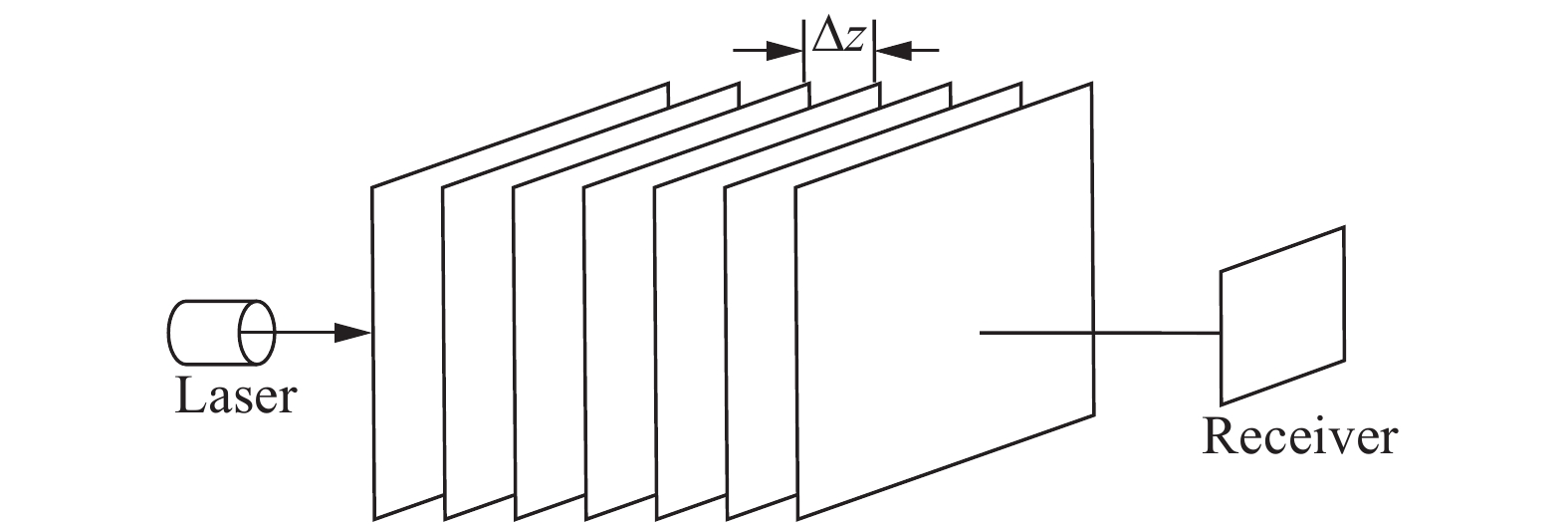
The principle of phase screen method ^[7]is considering the beam propagate through vacuum and phase screens along the transmission path alternately as shown inFig.1. The propagation distance L is divided into many parts, turbulence effects of each part is considered to be a phase screen, the light field between two adjacent phase screen can be expressed as

Here, $\Delta {z_{j + 1}} = {z_{j + 1}} - {z_j}$ is the distance between two phase screen located at ${z_{j + 1}}$ and ${z_j}$; ${\kappa _x}$ and ${\kappa _y}$ denotes the spatial frequency, the grids are divided to be $N \times N$ and the resolution is $\Delta x$, $F$ and ${F^{ - 1}}$ represents Fourier transform and Fourier inverse transform, respectively; $\varphi \left( {x,y} \right)$ reveals the phase fluctuation caused by turbulence which can be expressed as ^[7]

Here, $x = m\Delta x$, $y = m\Delta y$ represents the spatial domain, $\Delta x$, $\Delta y$ is the sample interval, m, n are integers; ${\kappa _x} = {m^{'}}\Delta {\kappa _x}$, ${\kappa _y} = {n^{'}}\Delta {\kappa _y}$ represents the frequency domain, $\Delta {\kappa _x}$, $\Delta {\kappa _y}$ is the sample interval, $m'$, $n'$ are integers; $a\left( {{\kappa _x},{\kappa _y}} \right)$ is the Fourier transform of the Gaussian random matrix with the mean value 0 and variance 1; ${\varPhi _\theta }\left( {{\kappa _x}{\rm{,}}\;{\kappa _y}} \right)$ represents the phase power spectrum, which is related to the power spectrum as

The parameter of phase screen mainly include the grid size $\Delta x$, screen size x and the number of phase screen along the propagation path N_PS. Since FFT method is usually used to calculate the beam propagation for program, the sample rule request is derived by Ref.[9]

Here, $\lambda $ is wavelength;L is the propagation distance. Considering that $x = \sqrt {\lambda LN} $, $\Delta x = \sqrt {\lambda L/N} $, the relationships between grid size $\Delta x$, screen size x and grids number N is decided. Usually the grids number N is decided firstly, and with higher N, the resolution of sample is more approximate while the computation complexity is higher. In this paper, the influence of different N is shown and compared.

Meanwhile, the description of beam should also be considered. For Gaussian beam, the beam width ${w_0}$ should be much bigger than $\Delta x$. Also, consider about the characteristics of turbulence, the sampling should be less than half of the coherence length $\Delta x \leqslant {r_0}/2$. Here the oceanic turbulence coherence length ${r_0} \approx 2.1{\rho _0}$^[10], spatial coherence scale ${\rho _0}$ for oceanic turbulence is derived by Ref.[11].

The number of phase screen along the path is decided by the turbulence strength. According to Ref.[12], the fluctuation between two phase screens should be small enough and meet the requirements of Rytov variance $\sigma _R^2\left( {\Delta z} \right) < 0.1$, then the requirement of phase screen number could be expressed as

Rytov variance $\sigma _R^2$ can be approximately expressed as^[13]:

The example of parameter settings is as follows:

(1) Consider about the strongest turbulence condition as an example, L=50 m, $\varepsilon = {10^{ - 6}}{{\rm{m}}^2}{{\rm{s}}^{ - 3}}$, ${\chi _T} = {10^{ - 6}}{K^2}{s^{ - 1}}$, $\omega = - 2$. Substituting into Eq.(14), ${r_0} \approx 0.7\;{\rm{mm}}$ is obtained. Consider that $\Delta x \leqslant {r_0}/2$, $\Delta x < < {w_0}$, the grid size should fulfill $\Delta x \leqslant 0.35\;{\rm{mm}}$, grids number should fulfill $N \geqslant 238$.

(2) Use Eq.(15) to calculate the phase screen number, and the distance between adjacent phase screens are should meet $\Delta z \leqslant 2.5$. During the simulation in this paper, the distance between screens is 2.5 m, which is much lower than the atmospheric turbulence simulation conditions.

Assuming that the long exposure intensity distribution is Gaussian, the statistical properties calculation could be expressed as ^[7]. Long exposure beam footprint radius:

Standard deviation of the fluctuation of the instantaneous center of the beam:

On-axis scintillation index:

Here, < > represents the average and ${{{r}}_c}$ is the position of beam center.

The following values of parameters are used in the calculations unless the statement of other values: wavelength $\lambda = 532\;{\rm{nm}}$, waist width ${w_0} = 10\;{\rm{mm}}$, inner scale $\eta = 1\;{\rm{mm}}$, $L = 10\;{\rm{m}}$, $\varepsilon = {10^{ - 6}}{{\rm{m}}^2}{{\rm{s}}^{ - 3}}$, $\omega = - 2$, ${\chi _T} = {10^{ - 6}}{K^2}{s^{ - 1}}$. According to the example show in Sect.3.2, the grids of phase screen is N=1024 and 2048, leading to the parameter setting $N = 1\;024,x = 0.16\;{\rm{m}}, \Delta x = 0.16\;{\rm{mm}}$ and $N = 2\;048$, $x = 0.24\;{\rm{m}}$, $\Delta x = 0.12\;{\rm{mm}}$, respectively. The distance between screens is 2.5 m. Note that the theory results are calculated by the expressions shown in Sec.2 and the numerical simulation results is obtained by the expressions in Sec.3.3 after the average of 1000 realizations.

The results presented in Fig.2(a) and 2(b) reveal that using phase screen method can achieve good correspondence between theoretical and numerical calculations of such statistical characteristics as long-exposure beam radius W_LE and ${\sigma _c}$ on the basis of appropriate parameter setting. Higher resolution numerical grid (2048 × 2 048 pixels) leads to better accuracy and longer distance weaken the correspondence. However, Fig.2(c) shows that the scintillation index $\sigma _I^2$, which represents the statistical characteristics of second moment of intensity, only have good agreement between theory and numerical results in short distance propagation and the increasement of grids does not make much change to the results.

Fig. 3-5 shows the similar tendency as Fig.2 that the analytical formula and phase screen numerical simulation for beam spreading and beam wander of Gaussian beam through oceanic turbulence are in good agreements under different turbulence conditions. The simulation results tends to be more approximate when the grids resolution gets higher. Figures also reveal that ${W_{{{LE}}}}$ and ${\sigma _c}$ increase when turbulence gets stronger (higher dissipation of mean-squared temperature ${\chi _T}$, lower rate of dissipation of kinetic energy per unit mass of seawater $\varepsilon $ and higher ratio of temperature to salinity contribution $\omega $). However, stronger turbulence affects consistency of the simulation results while the inconsistency keeps under 10%, which illustrates that phase screen method is suitable for being used under different turbulence conditions.

Similar to the results in Fig.2, the on-axis scintillation index $\sigma _I^2$ show good match in weak fluctuation regime, the error keeps increase when the turbulence gets stronger $\sigma _I^2 > 1$. The similar significant mismatch between numerical simulations and theoretical results for the scintillation index have been reported in earlier works about atmospheric turbulence. The reason is explained as the impact of either inner scale effect^[14-15] or beam wander induced scintillations^[16]. Ref.[12] proves that the major reason for this mismatch is the irregular appearance of large-amplitude (giant) irradiance spikes whose amplitudes greatly exceed the diffraction-limited peaks.

In this paper, the analytical formulas of beam spreading, beam wander and scintillation of Gaussian beam through oceanic turbulence are derived. The principle of parameter setting for phase screen simulated oceanic turbulence is mainly discussed and the steps are given in Sec.2.2. Furthermore, the comparison of the simulation results and theory calculation under different parameter settings and different turbulence conditions are shown in figures.

Results show that beam spreading and beam wander characteristics simulated by phase screen method are in good accordance with the theory formula under different turbulence conditions while the scintillation index has large deviation under strong fluctuation turbulence conditions. In summary, based on appropriate parameter setting, phase screen method can be a simple and effective way to calculate the statistical characteristics depend on the first moment of intensity, such as beam spreading and beam wander. The statistical characteristics depend on the second moment of intensity calculated by numerical simulation achieve good correspondence with theory in weak fluctuation regime and big mismatch in strong fluctuation regime, which should be further researched in the future.

References

[1] Y Li, L Yu, Y Zhang. Influence of anisotropic turbulence on the orbital angular momentum modes of Hermite-Gaussian vortex beam in the ocean. Optics Express, 25, 12203(2017).
[2] D Li, D Deng, F Zhao. Propagation properties of spatiotemporal chirped Airy Gaussian vortex wave packets in a quadratic index medium. Optics Express, 25, 13527(2017).
[3] Chenlu Xu, Shiqi Hao, Dai Zhang. Design of atmospheric turbulence phase screen set under the influence of combined oblique propagation and beam propagation. Infrared and Laser Engineering, 48, 0404003(2019).
[4] Dun Li, Yu Ning, Wuming Wu. Numerical simulation and verification of dynamic atmospheric turbulence with rotating phase screens. Infrared and Laser Engineering, 46, 1211003(2017).
[5] T Yang, S Zhao. Study on the Model of Ocean Turbulence Random Phase Screen. Acta Optica Sinica, 37, 1201001(2017).
[6] Chaojun Niu, Fang Lu, Xiang'e Han. Propagation properties of Gaussian array beams transmitted in oceanic turbulence simulated by phase screen method. Acta Optica Sinica, 38, 0601004(2018).
[7] rews L, Phillips R. Laser Beam Propagation Through Rom Media[M]. Bellingham: SPIE Press, 2005.
[8] V V Nikishov, V I Nikishov. Spectrum of turbulent fluctuations of the sea-water refraction index. Fluid Mechanics Research, 27, 82-98(2000).
[9] D Voelz, M Roggemann. Digital simulation of scalar optical diffraction: revisiting chirp function sampling criteria and consequences. Applied Optics, 48, 6132-6142(2009).
[10] D Fried. Optical resolution through a randomly inhomogeneous medium for very long and very short exposures. JOSA A, 56, 1372-1379(1966).
[11] L Lu, X Ji, Y Baykal. Wave structure function and spatial coherence radius of plane and spherical waves propagating through oceanic turbulence. Optics Express, 22, 27112-27122(2014).
[12] S Lachinova, M Vorontsov. Giant irradiance spikes in laser beam propagation in volume turbulence: analysis and impact. Journal of Optics, 18, 025608(2016).
[13] Lu Lu. Influence of oceanic turbulence on propagation of laser beams[D]. Hefei:University of Science Technology of China, 2016: 5256.(in Chinese)
[14] S M Flatte, G Y Wang, J Martin. Irradiance variance of optical waves through atmospheric turbulence by numerical simulation and comparison with experiment. JOSA A, 10, 2363-2370(1993).
[15] A Consortini, F Cochetti, J H Churnside. Inner-scale effect on irradiance variance measured for weak-to-strong atmospheric scintillation. JOSA A, 10, 2354-2362(1993).
[16] L Andrews, R Phillips, L Ronald. Strehl ratio and scintillation theory for uplink Gaussian-beam waves: beam wander effects. Optical Engineering, 45, 076001(2006).