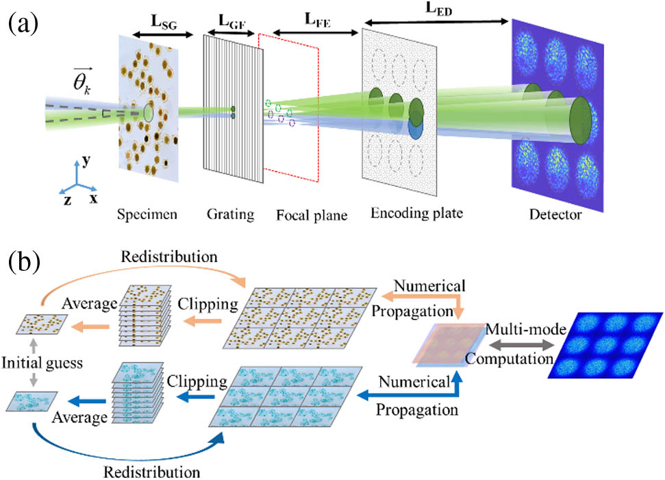
Fig. 1. (a) Schematic diagram of the principle of SUM–CDI. (b) Data flow chart of SUM–CDI.

Fig. 2. Iterative computation method of SUM–CDI.

Fig. 3. (a) Optical path diagram of the SUM–CDI experimental system. (b) Amplitude distribution of the encoding plate. (c) Phase distribution of the encoding plate. The units of the color bar of (c) are in radians. The scale bar in (b) is applicable to (c).

Fig. 4. (a) Time sequence diagram of probe pulse sequence and pump pulse in single-shot mode. (b) Intensity diagram of diffraction pattern in shot 1. (c) Amplitude distribution of the specimen at the corresponding time of each frame reconstructed by SUM–CDI. (d) Phase distribution of the specimen at the corresponding time of each frame reconstructed by SUM–CDI. The units of the color bar of phase in (d) are in radians. The scale bar in (c) is applicable to (d).

Fig. 5. Phase curves in (a) Shot 1, (b) Shot 2, and (c) Shot 3. The phase curves are plotted along blue broken lines in Fig. 4(d).

Fig. 6. Experimental result on spatial resolving capability. (a1)–(a4) Diffraction patterns recorded separately, and (a5) hybrid diffraction pattern by adding (a1)–(a4) together. (b1)–(b4) Images reconstructed from (a1)–(a4), respectively. (c1)–(c4) Reconstructed images from (a5) with SUM–CDI. (d1)–(d4) Resolution comparison between (c1)–(c4) and (b1)–(b4), respectively.

Fig. 7. Experimental results on accuracy in phase object imaging. (a1)–(a4) Diffraction patterns recorded separately, and (a5) hybrid diffraction pattern by adding (a1)–(a4) together. (b1)–(b4) Images reconstructed from (a1)–(a4), respectively. (c1)–(c4) Reconstructed images from (a5) with SUM–CDI. (d1)–(d4) Accuracy comparison between (c1)–(c4) and (b1)–(b4), respectively. The units of the color bar are in radians.

Fig. 8. (a)–(d) Amplitude and (e)–(h) phase of the specimen corresponding to different times T. The units of the colorbar are in radians. The scale bar in (a) is applicable to (b)–(h).

Fig. 9. (a), (b) Diffraction patterns of multiplexed CMI and SUM–CDI, respectively. (c), (d) Distributions of light on focal planes of multiplexed CMI and SUM–CDI, respectively.

Fig. 10. Reconstructed amplitude and phase. (a), (b) Four reconstructed amplitudes and four reconstructed phases of multiplexed CMI with diffraction patterns in Fig. 9(a), respectively. (c), (d) Four reconstructed amplitudes and four reconstructed phases of SUM–CDI with diffraction patterns in Fig. 9(b), respectively. (e) SNR curves for multiplexed CMI and SUM–CDI reconstruction results. The units of the colorbar are in radians. The scale bar in (a) is applicable to (b)–(d).

Fig. 11. (a) Diffraction patterns recorded by the detector at different times with an interval of 2 s and each pattern contains four subpatterns corresponding to four pulse probes. (b)–(e) Corresponding subpatterns extracted from (a) with SUM–CDI. The scale bar in (a) is applicable to (b)–(e).

Fig. 12. Experiment results of USAF 1951 (a)–(e) amplitude and (f)–(j) phase test target without the Dammann grating. (a) and (f) Diffraction patterns recorded by the detector. (b) and (g) Focus spots reconstructed from (a) and (f), respectively. (c) and (h) Corresponding retrieved amplitudes and phase distributions. (d) and (i) Enlarged views of the red boxes. (e) and (j) 1D curves of the blue lines. The unit of the colorbar is in radians.