Single-shot ultrafast multiplexed coherent diffraction imaging

Yingming Xu; Xingchen Pan; Mingying Sun; Wenfeng Liu; Cheng Liu; Jianqiang Zhu

doi:10.1364/PRJ.460948

Abstract

Classic interferometry was commonly adopted to realize ultrafast phase imaging using pulsed lasers; however, the reference beam required makes the optical structure of the imaging system very complex, and high temporal resolution was reached by sacrificing spatial resolution. This study presents a type of single-shot ultrafast multiplexed coherent diffraction imaging technique to realize ultrafast phase imaging with both high spatial and temporal resolutions using a simple optical setup, and temporal resolution of nanosecond to femtosecond scale can be realized using lasers of different pulse durations. This technique applies a multiplexed algorithm to avoid the data division in space domain or frequency domain and greatly improves the spatial resolution. The advantages of this proposed technique on both the simple optical structure and high image quality were demonstrated by imaging the generation and evaluating the laser-induced damage and accompanying phenomenon of laser filament and shock wave at a spatial resolution better than 6.96 μm and a temporal resolution better than 10 ns.

1. INTRODUCTION

Ultrafast imaging is extremely important for measuring unrepeatable transient phenomena, such as the propagation of shock wave [1], laser-induced damage [2], and exciton diffusion [3], which were difficult to measure with a common video camera. Compared to a traditional mechanical ultrafast camera that improves imaging speed by reducing the exposure time of detector [4 –6], most ultrafast imaging techniques reconstruct a sequence of images from one frame of data recorded with single detector exposure [7 –10]. Ultrafast imaging can generate both intensity and phase images depending on the optical alignment and the reconstruction algorithm applied [9,11 –13] and, generally speaking, ultrafast phase imaging is more sensitive and suitable for observation of transparent dynamic samples such as laser plasma [13 –15] and shock wave [16,17]. Compressed ultrafast photography (CUP) is the fastest intensity imaging technique used now. It applies a strategy of compressive sensing and can reach the speed of 10 trillion frames per second (Tfps) in imaging a sparse-enough sample [18 –20]. Ultrafast phase imaging was commonly realized using the strategy of ultrafast interferometry [9], where multilaser pulses illuminate a sample sequentially and interfere with an additional reference beam. Then the interferogram formed was recorded with single detector exposure. When the polarization or incident angle of each illuminating pulse is different, the phase and amplitude of all laser pulses leaving the sample at slightly different times can be separately numerically reconstructed. The highest temporal resolution of this interferometry-based ultrafast phase imaging technique is 1.6 ns; however, the reference beam adopted makes the optical alignment of interferometry-based ultrafast phase imaging quite complex, which seriously limits its application. On the other hand, since the interferogram of each illuminating laser pulse occupies only a small region in spatial domain or frequency domain, the achieved spatial resolution is inversely proportional to the number of illuminating laser pulses.

Coherent diffraction imaging (CDI) was mainly developed for short wavelengths, including X-rays [21,22] and high energy electron beams [23,24], where high-quality optical elements are not available. CDI can reach diffraction-limited resolution via iterative reconstructing approaches [25,26]. The outstanding advantage of CDI lies in its capability to realize phase imaging with simple optical alignment, and the accuracy and image quality of CDI are now comparable to that of traditional interferometry and holography, even in the regime of visible light. Several researches have illustrated the possibility of using CDI to replace interferometry to realize ultrafast phase imaging with a compact optical structure [27,28]. However, since each recorded subdiffraction pattern occupies only a small region of the sensing chip, CDI-based ultrafast phase imaging suffers from degradation in the spatial resolution. In other words, time-resolved phase imaging was realized with CDI at the cost of low spatial resolution, reducing its applicability for circumstances that require both high spatial and temporal resolutions.

A multimode CDI algorithm [29 –31] that takes full advantages of the information redundancy involved in diffraction intensity provides a new approach to circumvent the problem of degradation in the spatial resolution in CDI-based ultrafast phase imaging. This paper proposes a kind of single-shot ultrafast multiplexed CDI (SUM–CDI) to realize quantitative ultrafast phase imaging without degradation in the spatial resolution. Several laser pulses illuminate the sample under inspection in sequence, and diffraction pattern arrays formed by each laser pulse that arrive at the sensor chip at different times are recorded with a single detector exposure. Then, time-resolved images can be reconstructed using a specially designed multiplexed CDI algorithm. The temporal resolution of this proposed method was determined by the pulse duration of the illuminating pulses, which was changeable in a range from microseconds to femtoseconds. On the other hand, since the diffraction patterns formed by each illuminating laser pulse occupy the entire sensor chip of the detector, the reconstructed images have high-enough temporal and spatial resolutions. The performance of this proposed approach was verified by imaging the generation and evolution of laser-induced damage and the accompanying phenomenon of laser filament and shock wave inside K9 glass at a temporal resolution of 10 ns and a spatial resolution of 6.96 μm. The temporal resolution can be improved further to picoseconds or femtoseconds by using shorter laser pulses for illumination, and its spatial resolution can be improved further by using a larger sensor chip. To the best of our knowledge, this is the first time that single-shot ultrafast phase imaging with multiplexed CDI has been realized and used to experimentally measure unrepeatable transient process.

Sign up for Photonics Research TOC. Get the latest issue of Photonics Research delivered right to you！Sign up now

2. PRINCIPLE

The principle of the proposed SUM–CDI was schematically shown in Fig. 1(a), where several focused laser pulses illuminate a specimen at incident angles of $\vec{θ_{k}} = {(θ_{k}^{x}, θ_{k}^{y}) |}_{k = 1, \dots, K}$ , and the $k$ th laser pulse arriving at the grating in the $x^{'} y^{'}$ plane is $G_{k} (x^{'}, y^{'}) e^{i 2 π (x^{'} \frac{\cos θ_{k}^{x}}{λ} + y^{'} \frac{\cos θ_{k}^{x}}{λ})}$ , and its transmitted light was split into a beam cluster, which is denoted as ${G_{k} (x^{'}, y^{'}) e^{i 2 π [x^{'} \frac{\cos (α_{m_{x}} + θ_{k}^{x})}{λ} + y^{'} \frac{\cos (β_{m_{y}} + θ_{k}^{y})}{λ}]} |}_{m_{x} = 1, \dots, M_{1}, m_{y} = 1, \dots, M_{2}}$ . Then, this cluster of laser beams is incident on the encoding plate and forms complex diffraction patterns of $D_{k} (x, y)$ on the detector, where each $D_{k} (x, y)$ was composed of $M = M_{1} \times M_{2}$ partially overlapped diffraction disks.

(a) Schematic diagram of the principle of SUM–CDI. (b) Data flow chart of SUM–CDI.

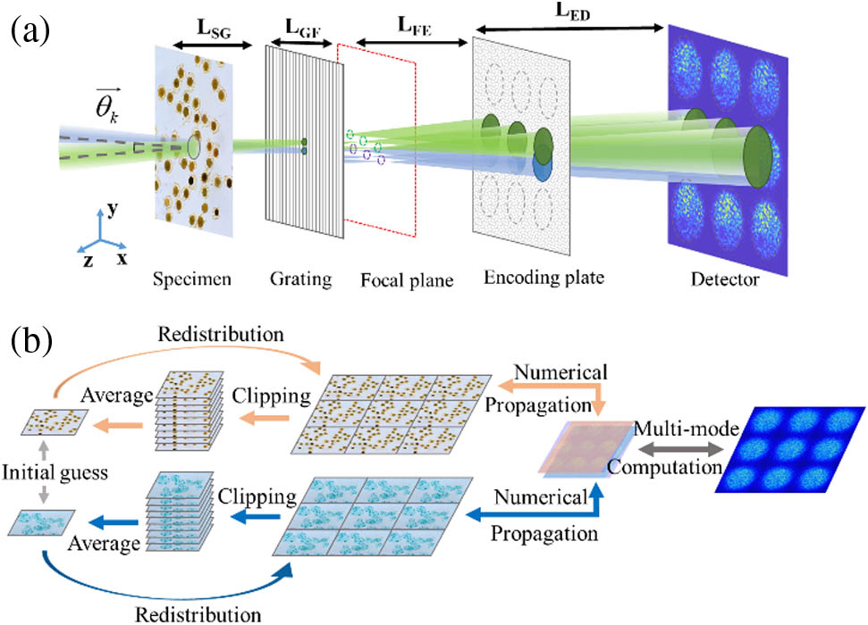
Figure 1.(a) Schematic diagram of the principle of SUM–CDI. (b) Data flow chart of SUM–CDI.

When there is only one illuminating pulse, $M$ complex images on the specimen plane can be reconstructed with a common coherent modulation imaging (CMI) algorithm [32,33]. Since all these images are the same in theory, the SNR of a reconstructed image can be effectively improved by doing an average on these $M$ images in each iteration; this is the underlying physics for the split-coding method to be better than common CMI. For simplicity, only two illumination pulses are schematically drawn in Fig. 1(a), and in an experiment the number of illumination pulses can be increased to 10 or more to split the transient process into 10 or more temporal slices.

When a series of laser pulses are incident on a specimen at times of $t_{k} = {t_{0} + k Δ t |}_{k = 1, \dots, K}$ , the recorded diffraction pattern can be written as $I (x, y) = \sum_{k = 1}^{K} {| D_{k} (x, y) |}^{2}$ . By using a multimode reconstructing algorithm with consideration on the specific incident angle ${(θ_{k}^{x}, θ_{k}^{y}) |}_{k = 1, \dots, K}$ for each illumination pulse, ${G_{k} (x^{'}, y^{'}) |}_{k = 1, \dots, K}$ corresponding to the property of specimen at times of $t_{k} = {t_{0} + k Δ t |}_{k = 1, \dots, K}$ can be reconstructed separately.

Figure 1(b) shows the reconstructing data flow chart of this proposed method corresponding to Fig. 1(a). After giving two initial guesses to two images of $O_{1} (x, y)$ and $O_{2} (x, y)$ , which correspond to two states of specimen at $t_{1} = t_{0} + Δ t$ and $t_{2} = t_{0} + 2 Δ t$ , respectively, nine replicas of reconstructed $O_{1} (x, y)$ and $O_{2} (x, y)$ can be generated by forward and backward propagating light beams between specimen plane and detector plane via the encoding plate iteratively using a multimode algorithm. Since the diffraction pattern is not segmented, high-frequency information is preserved under the premise of ensuring multimode measurement. In each iteration, nine replicas corresponding to each illuminating pulse were replaced with their averages to improve the reconstruction accuracy. Finally, $O_{1} (x, y)$ and $O_{2} (x, y)$ of high accuracy are reconstructed after enough iteration times.

3. COMPUTATION METHOD

The computing method is shown in Fig. 2, where an initial guess was given to each probing laser pulse arriving at encoding plate as $E_{k} (x, y)$ , and an iterative computation was carried out with the following steps. (1)Calculate the transmitted field of each probe laser pulse leaving the encoding plate and its diffraction patterns $D_{k} (X, Y)$ formed on detector plane with $D_{k} (X, Y) = F [E_{k} (x, y) \cdot T (x, y), L_{ED}], k = 1, 2, \dots, K,$ (1)where $T (x, y)$ is the transmitting function of encoding plate, and $E_{k} (x, y) \cdot T (x, y)$ is the transmitted light of the $k$ th probe laser pulse. $F [E_{k} (x, y) \cdot T (x, y), L]$ represents the forward propagation of $E_{k} (x, y) \cdot T (x, y)$ by a distance of $L$ with a Fresnel formula.(2)Calculate the reconstruction error on the detector plane with $Error = \frac{| \sum_{k = 1}^{K} {| D_{k} (X, Y) |}^{2} - I (X, Y) |}{I (X, Y)} .$ (2)If the value of the computed error is smaller than the expected value, the iterative computation stops, or else jumps to step (3).1/Error can be used to represent the relative SNR value of the reconstruction results.(3)Update the diffraction patterns of all probe pulses with $D_{k}^{'} (X, Y) = \frac{\sqrt{I (X, Y)}}{\sqrt{\sum_{k = 1}^{K} {| D_{k} (X, Y) |}^{2}}} D_{k} (X, Y) .$ (3)(4)Back propagate each $D_{k}^{'} (X, Y)$ to the encoding plate plane with $φ_{k}^{'} (x, y) = F [D_{k}^{'} (X, Y), - L_{ED}] .$ (4)(5)Update the light field of each probe laser pulse illuminating on the encoding plate with $E_{k}^{'} (x, y) = E_{k} (x, y) + χ \frac{conj (T (x, y)) \cdot (φ_{k}^{'} (x, y) - φ_{k} (x, y))}{\max (\max (conj (T (x, y)) \cdot T (x, y)))},$ (5)where $χ$ is a constant in the range of [0,1] to adjust the updating speed.(6)Back propagate each $E_{k}^{'} (x, y)$ to the focal plane in Fig. 1 with $F_{k} (u_{0}, v_{0}) = F [E_{k}^{'} (x, y), - L_{FE}] .$ (6)Just as shown in Fig. 1, $F_{k} (u_{0}, v_{0})$ essentially is composed of $M$ separated focal spots corresponding to $M$ sub-beams; that is, $F_{k} (u_{0}, v_{0})$ should be written as $F_{k m} (u_{0}, v_{0}) |_{k = 1, \cdot \cdot \cdot, K, m = 1, \cdot \cdot \cdot, M}$ .(7)Use the spatial constrain $H_{k m} (u_{0}, v_{0}, a_{k m}, b_{k m})$ in $H_{k m} (u_{0}, v_{0}, a_{k m}, b_{k m}) = {\begin{matrix} 1 & {(u_{0} - a_{k m})}^{2} + {(v_{0} - b_{k m})}^{2} < R^{2} \\ 0 & {(u_{0} - a_{k m})}^{2} + {(v_{0} - b_{k m})}^{2} > R^{2} \end{matrix}$ (7)to filter the focal spot array $F_{k m} (u_{0}, v_{0})$ , and propagate them to the specimen plane as $A_{k m} (u_{0}, v_{0}) = F [H_{k m} (u, v, a_{k m}, b_{k m}) \cdot F_{k m} (u, v), - L_{FA}]$ , where $L_{FA}$ is the distance from focal plane to the average plane (specimen plane or imaging plane of specimen).Since each probing beam is incident on the sample at a slightly different angle, $a_{k m}$ and $b_{k m}$ change with respect to the specific incident angle. The value of $R$ is dependent on the diffraction angle of the Dammann grating and, after large enough number of iterations, the value of $R$ can take a very large value.(8) $A_{k m} (u_{0}, v_{0})$ includes $M$ separated replicas of the reconstructed specimen for each probe laser pulse, and, in theory, the relationship among them is $A_{k m} (u_{0}, v_{0}) = A_{k 0} (u_{0} - ξ_{k m}, v_{0} - η_{k m})$ . However, because of experimental factors, the noise in these replicas is quite different, and doing an average on them with $A_{k m} (u_{0}, v_{0}) = \frac{{sum}_{m} (| A_{k m} (u_{0}, v_{0}) |)}{\sum_{m = 1}^{M} {sum}_{m} (| A_{k m} (u_{0}, v_{0}) |)} \sum_{m = 1}^{M \times M} A_{k m} (u_{0}, v_{0})$ (8)can effectively reduce the noise and improve reconstruction quality. In Eq. (8), ${sum}_{m} (\cdot)$ represents element value of $m$ th specimen replicas to be summed.(9)Redistribute $A_{k m} (u_{0}, v_{0})$ with Eq. (9) and get updated $E_{k} (x, y)$ as $E_{k} (x, y) = F [\sum_{m = 1}^{M} A_{k m} (u_{0} + ξ_{k m}, v_{0} + η_{k m}), L_{AE}],$ (9)where $L_{AE}$ is the distance from the average plane to the encoding plate plane.

Figure 2.Iterative computation method of SUM–CDI.

4. EXPERIMENTAL RESULTS

Optical alignment. The suggested SUM–CDI was applied to observe the evaluation of laser-induced damage in K9 glass as well as the accompanying phenomenon of laser filament and shock wave. The optical alignment used is shown in Fig. 3, where a nanosecond laser pulse with a wavelength of 1064 nm and pulse duration of 8 ns is frequency-doubled by the crystal BBO-1 and then frequency-tripled by crystal BBO-2 to generate new wavelengths of 355 nm and 532 nm. A laser pulse of 355 nm illuminates a piece of K9 glass to generate laser-induced damage. The laser pulse of 532 nm is split into four beams by a fiber coupler and then propagates separately in four single-mode fibers of different lengths to introduce a temporal interval of 10 ns among them. The output ends of these four fibers are at the front focal plane of lens-3, and then the specimen is illuminated by four parallel laser beams at slightly different incident angles. The angular interval between two adjacent illuminating laser pulses incident on specimen is 0.2 deg. The amplitude and phase distributions of the encoding plate used in the experiment are shown in Figs. 3(b) and 3(c), which are measured by an extended ptychographic iterative engine (ePIE), and the encoding plate is a random $0 - π$ binary phase plate with element size of $100 μm \times 100 μm$ . Lens-4 is applied to magnify the specimen to improve the spatial resolution of finally reconstructed images. The Dammann grating splits each probe pulse into $3 \times 3$ replicas (the separation angle is 0.5 deg), the diffraction patterns $D_{k} (x, y)$ formed on detector are composed of $3 \times 3$ diffraction disks, and the recorded intensity is the summation of four frames of diffraction intensities corresponding to four probe pulses; that is, $I (x, y) = \sum_{k = 1}^{4} {| D_{k} (x, y) |}^{2}$ . The detector is a 16-bit scientific CMOS camera (pco.edge 4.2. PCO GmbH) with $2048 \times 2048$ pixels, and the size of each pixel is $6.5 μm \times 6.5 μm$ .

Figure 3.(a) Optical path diagram of the SUM–CDI experimental system. (b) Amplitude distribution of the encoding plate. (c) Phase distribution of the encoding plate. The units of the color bar of (c) are in radians. The scale bar in (b) is applicable to (c).

Measurement result. Damage induced by the nanosecond laser pulse inside K9 glass was always accompanied by various physics phenomena, including laser filament, laser plasma, shock wave, thermal ablation, plume expansion, and crack formation [34 –39]. These phenomena affect the amplitude and phase of the light beam transmitting damaged volume. Correspondingly, by doing ultrafast imaging with the SUM–CDI method illustrated above, the evolution of laser-induced damage and accompanying phenomenon can be measured with single detector exposure.

The temporal intervals among four probe laser pulses of 532 nm and one pump pulse of 352 nm are shown in Fig. 4(a), where the first probe pulse arrives at the specimen about 10.2 ns earlier than the pump pulse. The second probe pulse and the pump pulse arrive at the specimen simultaneously, and the pump pulse causes damage in K9 glass. The temporal intervals of the third probe pulse to the second and the fourth ones are 16.8 ns and 11.5 ns, respectively. Thus, the first probe reveals the original state of specimen, and the second probe reveals the state of the specimen during the interaction between the pump laser pulse and glass, and the third and the fourth pulses show the evaluation of damage after the finish of laser-material interaction. The temporal resolution of this suggested SUM–CDI in Fig. 3 was about 10 ns, and it depends on the pulse duration of the probe pulse. The energy density of pump pulse $152.8 J / {cm}^{2}$ , is 3.8 times the damage threshold of K9 glass. One recorded diffraction intensity $I (x, y) = \sum_{k = 1}^{4} {| D_{k} (x, y) |}^{2}$ is shown in Fig. 4(b), where there are $3 \times 3$ partially overlapped diffraction disks, and the separation of four diffraction patterns corresponding to four probe laser pulses is shown in Appendix B.

$(a) Time sequence diagram of probe pulse sequence and pump pulse in single-shot mode. (b) Intensity diagram of diffraction pattern in shot 1. (c) Amplitude distribution of the specimen at the corresponding time of each frame reconstructed by SUM–CDI. (d) Phase distribution of the specimen at the corresponding time of each frame reconstructed by SUM–CDI. The units of the color bar of phase in (d) are in radians. The scale bar in (c) is applicable to (d).$

Figure 4.(a) Time sequence diagram of probe pulse sequence and pump pulse in single-shot mode. (b) Intensity diagram of diffraction pattern in shot 1. (c) Amplitude distribution of the specimen at the corresponding time of each frame reconstructed by SUM–CDI. (d) Phase distribution of the specimen at the corresponding time of each frame reconstructed by SUM–CDI. The units of the color bar of phase in (d) are in radians. The scale bar in (c) is applicable to (d).

From the recorded diffraction patterns shown in Fig. 4(b), the intensity and phase of four transmitted probe pulses are reconstructed and shown in the first line of Fig. 4(c) and Fig. 4(d), respectively. K9 glass is uniform in both the refractive index and surface profile before the arrival of a pump pulse; thus, the reconstructed intensity and phase images corresponding to the initial state of specimen at the time of $- 10.2 ns$ both have uniform values, as shown in image 1-1 and image 1-5. The reconstructed intensity and phase images of the second probe pulse, which arrives at the specimen at $t = 0 ns$ , are shown in image 1-2 and image 1-6, respectively. The interaction between the strong pump pulse field and K9 glass changes the refractive index and surface profile of glass plate. The small black spot at the center of image 1-2 is a tiny damage cave on glass surface. The bright line in phase image 1-6 indicates the laser filament [38]. At $t = 16.8 ns$ and $t = 28.3 ns$ the pump pulse has left the silica glass; however, the formed laser filament shown as bright lines in images 1-7 and 1-8 is still remarkable. Two bright rings in image 1-7 and image 1-8 correspond to wave fronts of generated shock wave, and the phase values inside theses ring are obviously smaller than the phase values outside them. This is due to the contribution of free electrons to the optical refractive index [40]. After two seconds, when the change of specimen caused by the first pump pulse stops, the second pump pulse hits the specimen at the same position of the first pump pulse, and the second frame of diffraction patterns is recorded. The reconstructed intensity and phase images are shown in the second line in Figs. 4(c) and 4(d). After another two seconds, the third pump pulse hits the specimen at the same position again, and the third frame of diffraction patterns is recorded. The reconstructed intensity and phase images are shown in the third line in Figs. 4(c) and 4(d). Because of the existence of damages generated by previous pump pulses, the laser filament that consumes some ratio of laser energy does not take place in the images of 2-7, 2-8, 3-7, and 3-8, then the energy of the formed shock wave is larger than that in images 1-7 and 1-8, resulting in a faster propagation speed [15,16]. This is the reason why the diameters of bright rings in the second and third lines are slightly larger than in the first line. These experimental results match theoretical predictions well and sufficiently prove the feasibility of the proposed SUM–CDI.

To further check the correctness of measurements above, the speed of the shock wave was calculated using the experimental results above. The values of the reconstructed phase images corresponding to three pump pulses are plotted along the blue broken lines and shown in Figs. 5(a), 5(b), and 5(c), respectively. In Fig. 4(d), the 12 subfigures use one colorbar, and the background value is unified to the minimum value. Therefore, the phase range of the 1D curve in Fig. 5 is less than $[- 4, 3]$ . In Fig. 5, $P_{0}$ corresponds to the center of the damage spot, and $P_{m}^{k}$ corresponds the position of the generated shock wavefront in the kth reconstructed phase image of the specimen under the illumination of the mth pump laser pulse. According to Sedov’s blast wave theory, the diameter of a spherical shock wavefront is $r = α {(\frac{2.35 E}{ρ})}^{1 / 5} t^{\frac{2}{5}}$ [41,42], where $α$ is a constant roughly equal to 1, $E$ is the energy that drives the shock wave, and $ρ$ is the density of undisturbed air. By taking the values of $ρ = 1.2 kg / m^{3}$ , $α = 1.0$ , and the distance of $P_{0}$ to $P_{1}^{2}$ in Fig. 5(a) measured as 83 μm, the energy $E$ of shock wave can be computed as 7.1 μJ. With this calculated $E$ , the distance between $P_{0} and P_{1}^{3}$ predicted by $r = α {(\frac{2.35 E}{ρ})}^{1 / 5} t^{\frac{2}{5}}$ is 102 μm. Compared to the distance of 104 μm measured from Fig. 5(a), the error is only 2%. Similarly, energies of two shock waves generated by the 2nd and 3rd pump pulses can be computed as 19.1 μJ and 24.2 μJ, respectively, which both are slightly higher than that of the first pump pulse because no laser filament consumes laser energy in these two cases. The diameters of two generated spherical shock waves in image 2-8 and image 3-8 decided by $r = α {(\frac{2.35 E}{ρ})}^{1 / 5} t^{\frac{2}{5}}$ are 100 μm and 106 μm, respectively. Compared to the measured distances of $P_{2}^{3}$ and $P_{3}^{3}$ to $P_{0}$ in Figs. 5(b) and 5(c), the computing error is also about 2%. These computations and comparisons sufficiently prove the high accuracy of the proposed SUM–CDI in imaging highly transient processes.

Figure 5.Phase curves in (a) Shot 1, (b) Shot 2, and (c) Shot 3. The phase curves are plotted along blue broken lines in Fig. 4(d).

Spatial resolving capability. Compared to other ultrafast phase imaging methods, the outstanding advantage of the suggested SUM–CDI lies in its compact optical structure and high spatial resolution. In other words, time-resolved images are obtained using a simple optical setup without degradation in its spatial resolving capability. To demonstrate this advantage experimentally, another set of experiments were carried out using the resolution target of USAF 1951 as the specimen, and experimental results are shown in Fig. 5. By using four probe light beams to illuminate the specimen separately and acquiring four independent diffraction patterns $| D_{k} (x, y) |_{k = 1, 2, 3, 4}^{2}$ shown in Figs. 6(a1)–6(a4), four reconstructed images can be computed separately and shown in Figs. 6(b1)–6(b4). By adding these four diffraction patterns $| D_{k} (x, y) |_{k = 1, 2, 3, 4}^{2}$ together to get the hybrid diffraction pattern $I (x, y) = \sum_{k = 1}^{4} {| D_{k} (x, y) |}^{2}$ shown in Fig. 6(a5) and using the same computational method as what was applied in a previous experiment, four images are computed from $I (x, y)$ and shown in Figs. 6(c1)–6(c4). To qualitatively compare the spatial resolution of images obtained with a separate computation method to that obtained with SUM–CDI, intensities along red and blue lines are plotted as red and blue curves in Figs. 6(d1)–6(d4) correspondingly. We can find that there are almost no differences between each pair of curves, showing the advantage of SUM–CDI in maintaining good spatial resolution. Since tiny bars of two elements in group 6 are clearly distinguished, the spatial resolution achieved in above experiments at least is 6.96 μm. In addition, the reconstruction results using common CMI in this situation are shown in Appendix C, and the comparison results show that SUM–CDI can effectively reduce the reconstruction noise.

$Experimental result on spatial resolving capability. (a1)–(a4) Diffraction patterns recorded separately, and (a5) hybrid diffraction pattern by adding (a1)–(a4) together. (b1)–(b4) Images reconstructed from (a1)–(a4), respectively. (c1)–(c4) Reconstructed images from (a5) with SUM–CDI. (d1)–(d4) Resolution comparison between (c1)–(c4) and (b1)–(b4), respectively.$

Figure 6.Experimental result on spatial resolving capability. (a1)–(a4) Diffraction patterns recorded separately, and (a5) hybrid diffraction pattern by adding (a1)–(a4) together. (b1)–(b4) Images reconstructed from (a1)–(a4), respectively. (c1)–(c4) Reconstructed images from (a5) with SUM–CDI. (d1)–(d4) Resolution comparison between (c1)–(c4) and (b1)–(b4), respectively.

Accuracy in phase object imaging. To check the accuracy of the proposed SUM–CDI in phase object imaging, a phase resolution target was used as a specimen to repeat the experiment shown in Fig. 6, and the experimental results are shown in Fig. 7. Figures 7(a1)–7(a4) are recorded diffraction patterns, and Fig. 7(a5) is the hybrid diffraction pattern by adding Figs. 7(a1)–7(a4) together. Figures 7(b1)–6(b4) are phase images reconstructed from Figs. 7(a1)–6(a4), respectively. Figures 7(c1)–7(c4) are images reconstructed from Fig. 7(a5) with the proposed SUM–CDI method, and almost no visible difference can be found when comparing Figs. 7(b1)–7(b4) to Figs. 7(c1)–7(c4). To make a quantitative comparison on two sets of reconstructed images, the phase intensities along the red and blue dotted lines are plotted as two curves in Figs. 7(d1)–7(d4), respectively. By comparing the red curves to the corresponding blue curves, we find that the difference between them is much smaller than 1%, which shows the very high accuracy of the proposed SUM–CDI method in phase object imaging.

$Experimental results on accuracy in phase object imaging. (a1)–(a4) Diffraction patterns recorded separately, and (a5) hybrid diffraction pattern by adding (a1)–(a4) together. (b1)–(b4) Images reconstructed from (a1)–(a4), respectively. (c1)–(c4) Reconstructed images from (a5) with SUM–CDI. (d1)–(d4) Accuracy comparison between (c1)–(c4) and (b1)–(b4), respectively. The units of the color bar are in radians.$

Figure 7.Experimental results on accuracy in phase object imaging. (a1)–(a4) Diffraction patterns recorded separately, and (a5) hybrid diffraction pattern by adding (a1)–(a4) together. (b1)–(b4) Images reconstructed from (a1)–(a4), respectively. (c1)–(c4) Reconstructed images from (a5) with SUM–CDI. (d1)–(d4) Accuracy comparison between (c1)–(c4) and (b1)–(b4), respectively. The units of the color bar are in radians.

5. DISCUSSION

Different from existing ultrafast phase imaging techniques, SUM–CDI applies a multiplexed strategy to avoid the division in the spatial domain or frequency domain, so it can achieve ultrafast phase imaging with high temporal–spatial resolutions and high accuracy by using a simpler optical setup. Theoretically, by using a detector with a large enough sensor chip and high enough dynamic range, diffraction limited spatial resolution can be reached, and its temporal resolution is only decided by the time duration of probing laser beams. Thus, by using a 32 bit detector, temporal–spatial resolution much higher than that of the experiments above is reachable.

Advantages of SUM–CDI. The advantage of the proposed SUM–CDI technique lies in two aspects. The first aspect is the adoption of Dammann grating, which splits the laser beam under inspection into several replicas, and all replicas are modulated by different regions of a random phase plate. Thus, it is essentially a kind of multichannel coherent modulation imaging, and the average operation on all channels effectively reduces the noise and results in a reconstructed image of high SNR and high accuracy; this is the underline physics for SUM–CDI to work for ultrafast phase imaging. In addition, because the detector records the high-order items of the grating, more high-frequency information can be recorded, thereby improving the spatial resolution of the system. The second aspect lies in its simple optical alignment, where the time of each probing laser pulse arriving at sample is simply encoded into its incident angle, and then in iterative reconstruction their Fourier transforms emerge at different positions in the spatial frequency domain, making the separation of all reconstructed probing laser pulses easy. On the other hand, the adoption of grating in the optical alignment and averaging operation in the reconstruction process effectively improve the information redundancy in the recorded data and correspondingly speed up the convergence speed of iterative reconstruction. The comparison of the convergence and SNR between the proposed SUM–CDI and common CMI is shown in Appendix A.

Required optical parameters. In theory, to get high reconstruction quality and high convergence speed, each probing laser pulse should be split into a large enough number of sub-beams by the Dammann grating. On the other hand, to ensure a sufficient field of view (FOV), the angle interval between adjacent sublaser beams should be large enough and, theoretically, the larger the interval angles, the less the crosstalk of different modes, which can reduce the noise. Since iterative reconstruction is realized by computing the Fresnel diffraction, where a paraxial approximation is applied, the permitted angle of the outmost sub-beams with respect to the optical axis is only about 10 deg, depending on the pixel size of detector. In the experiments above, by considering these factors in combination, the angle interval between the adjacent grating sub-beams is 0.5 deg, the FOV diameter range is 700 μm, and the element size of the random phase plate is $100 μm \times 100 μm$ .

Temporal resolution achievable. The temporal resolution of the proposed method is only limited by the temporal duration of probing laser pulses; therefore, in theory, temporal resolutions from microseconds to femtoseconds or even attoseconds can be achieved. However, when the pulse duration is shorter than 10 fs, the probing light beam is not monochromatic light anymore, and a multimode algorithm should be applied in the spectral domain to do iterative computation, which requires more information redundancy in recorded diffraction patterns. On the other hand, to increase the information redundancy of the recorded diffraction patterns, each probing laser pulse should be split into more sub-beams. Then a detector with a larger sensor chip and no-paraxial reconstruction algorithm are required [43]. In other words, temporal resolution as high as femtoseconds and attoseconds is reachable by using a more complex optical alignment and reconstructing algorithm.

6. CONCLUSION

To realize a sequence of ultrafast phase and amplitude imaging with a single diffraction pattern, a new scheme SUM–CDI that includes a grating, a weak modulator, a detector, and phase retrieval algorithms is proposed in this paper. Due to the information redundancy introduced by multiple modulation and the multiplex phase retrieval algorithm inspired by ptychography and CMI, at least four wave modes, including phase and amplitude, can be iteratively retrieved at once with a higher SNR. When combining with an ultrafast probe sequence, SUM–CDI could be used as an excellent technique for single-shot ultrafast optical imaging, which was demonstrated by measuring laser-induced damage with a temporal resolution at the 10 ns level and a spatial resolution of 6.96 μm. Aside from the intensity evolution of the damage spot, the corresponding quantized phase information could also be observed accurately by SUM–CDI, which is crucial to investigate the mechanism of ultrafast laser-induced damage, including the generation, propagation, and confrontation of shock waves, something which is difficult for other techniques without the capability of phase imaging. In addition, the temporal resolution is restricted by the pulse duration of the probe pulse and the time interval between adjacent probes, leaving room for potential improvement in temporal resolution to a Tfps rate. In addition, being a form of CDI, the theoretical resolution limitation of SUM–CDI is $λ / 2$ for multiplexed phase imaging [44], considering that the NA of the detector is utilized by all modes, which is quite different from other multiple phase imaging techniques based on the space division of the detector. In general, SUM–CDI is a promising technique for single-shot ultrafast optical imaging that can be used in a variety of fields, especially where ultrafast phase imaging with high resolution is urgently required.

APPENDIX A: COMPARISON BETWEEN SUM–CDI AND MULTIPLEXED CMI

{{\vec{θ}}_{k} |}_{k = 1, \dots, K}

Figure 8.(a)–(d) Amplitude and (e)–(h) phase of the specimen corresponding to different times $T$ . The units of the colorbar are in radians. The scale bar in (a) is applicable to (b)–(h).

$(a), (b) Diffraction patterns of multiplexed CMI and SUM–CDI, respectively. (c), (d) Distributions of light on focal planes of multiplexed CMI and SUM–CDI, respectively.$

Figure 9.(a), (b) Diffraction patterns of multiplexed CMI and SUM–CDI, respectively. (c), (d) Distributions of light on focal planes of multiplexed CMI and SUM–CDI, respectively.

$Reconstructed amplitude and phase. (a), (b) Four reconstructed amplitudes and four reconstructed phases of multiplexed CMI with diffraction patterns in Fig. 9(a), respectively. (c), (d) Four reconstructed amplitudes and four reconstructed phases of SUM–CDI with diffraction patterns in Fig. 9(b), respectively. (e) SNR curves for multiplexed CMI and SUM–CDI reconstruction results. The units of the colorbar are in radians. The scale bar in (a) is applicable to (b)–(d).$

Figure 10.Reconstructed amplitude and phase. (a), (b) Four reconstructed amplitudes and four reconstructed phases of multiplexed CMI with diffraction patterns in Fig. 9(a), respectively. (c), (d) Four reconstructed amplitudes and four reconstructed phases of SUM–CDI with diffraction patterns in Fig. 9(b), respectively. (e) SNR curves for multiplexed CMI and SUM–CDI reconstruction results. The units of the colorbar are in radians. The scale bar in (a) is applicable to (b)–(d).

APPENDIX B: SEPARATION OF FOUR DIFFRACTION PATTERNS CORRESPONDING TO FOUR PROBE LASER PULSES

t = - 10.2 ns

$(a) Diffraction patterns recorded by the detector at different times with an interval of 2 s and each pattern contains four subpatterns corresponding to four pulse probes. (b)–(e) Corresponding subpatterns extracted from (a) with SUM–CDI. The scale bar in (a) is applicable to (b)–(e).$

Figure 11.(a) Diffraction patterns recorded by the detector at different times with an interval of 2 s and each pattern contains four subpatterns corresponding to four pulse probes. (b)–(e) Corresponding subpatterns extracted from (a) with SUM–CDI. The scale bar in (a) is applicable to (b)–(e).

APPENDIX C: RECONSTRUCTION USING MULTIPLEXED CMI ALGORITHM WITH USAF 1951

3 \times 3

$Experiment results of USAF 1951 (a)–(e) amplitude and (f)–(j) phase test target without the Dammann grating. (a) and (f) Diffraction patterns recorded by the detector. (b) and (g) Focus spots reconstructed from (a) and (f), respectively. (c) and (h) Corresponding retrieved amplitudes and phase distributions. (d) and (i) Enlarged views of the red boxes. (e) and (j) 1D curves of the blue lines. The unit of the colorbar is in radians.$

Figure 12.Experiment results of USAF 1951 (a)–(e) amplitude and (f)–(j) phase test target without the Dammann grating. (a) and (f) Diffraction patterns recorded by the detector. (b) and (g) Focus spots reconstructed from (a) and (f), respectively. (c) and (h) Corresponding retrieved amplitudes and phase distributions. (d) and (i) Enlarged views of the red boxes. (e) and (j) 1D curves of the blue lines. The unit of the colorbar is in radians.

References

[1] A. Schropp, R. Hoppe, V. Meier, J. Patommel, F. Seiboth, Y. Ping, D. G. Hicks, M. A. Beckwith, G. W. Collins, A. Higginbotham, J. S. Wark, H. J. Lee, B. Nagler, E. C. Galtier, B. Arnold, U. Zastrau, J. B. Hastings, C. G. Schroer. Imaging shock waves in diamond with both high temporal and spatial resolution at an XFEL. Sci. Rep., 5, 11089(2015).

[2] H. Yang, J. Cheng, Z. Liu, Q. Liu, L. Zhao, J. Wang, M. Chen. Dynamic behavior modeling of laser-induced damage initiated by surface defects on KDP crystals under nanosecond laser irradiation. Sci. Rep., 10, 500(2020).

[3] D. Giovanni, M. Righetto, Q. Zhang, J. W. M. Lim, S. Ramesh, T. C. Sum. Origins of the long-range exciton diffusion in perovskite nanocrystal films: photon recycling vs exciton hopping. Light Sci. Appl., 10, 2(2021).

[4] L. Lazovsky, D. Cismas, G. Allan, D. Given. CCD sensor and camera for 100 Mfps burst frame rate image capture. Proc. SPIE, 5787, 184-190(2005).

[5] V. Tiwari, M. A. Sutton, S. R. McNeill. Assessment of high speed imaging systems for 2D and 3D deformation measurements: methodology development and validation. Exp. Mech., 47, 561-579(2007).

[6] R. Kodama, K. Okada, Y. Kato. Development of a two-dimensional space-resolved high speed sampling camera. Rev. Sci. Instrum., 70, 625-628(1999).

[7] Z. Li, R. Zgadzaj, X. Wang, Y. Y. Chang, M. C. Downer. Single-shot tomographic movies of evolving light-velocity objects. Nat. Commun., 5, 3085(2014).

[8] K. Nakagawa, A. Iwasaki, Y. Oishi, R. Horisaki, A. Tsukamoto, A. Nakamura, K. Hirosawa, H. Liao, T. Ushida, K. Goda, F. Kannari, I. Sakuma. Sequentially timed all-optical mapping photography (STAMP). Nat. Photonics, 8, 695-700(2014).

[9] Q.-Y. Yue, Z.-J. Cheng, L. Han, Y. Yang, C.-S. Guo. One-shot time-resolved holographic polarization microscopy for imaging laser-induced ultrafast phenomena. Opt. Express, 25, 14182-14191(2017).

[10] X. Wang, L. Yan, J. Si, S. Matsuo, H. Xu, X. Hou. High-frame-rate observation of single femtosecond laser pulse propagation in fused silica using an echelon and optical polarigraphy technique. Appl. Opt., 53, 8395-8399(2014).

[11] H. Hu, T. Liu, H. Zhai. Comparison of femtosecond laser ablation of aluminum in water and in air by time-resolved optical diagnosis. Opt. Express, 23, 628-635(2015).

[12] A. Barty, S. Boutet, M. J. Bogan, S. Hau-Riege, S. Marchesini, K. Sokolowski-Tinten, N. Stojanovic, R. Tobey, H. Ehrke, A. Cavalleri, S. Düsterer, M. Frank, S. Bajt, B. W. Woods, M. M. Seibert, J. Hajdu, R. Treusch, H. N. Chapman. Ultrafast single-shot diffraction imaging of nanoscale dynamics. Nat. Photonics, 2, 415-419(2008).

[13] J. Barolak, D. Goldberger, C. Durfee, D. Adams. Single-shot ptychographic imaging of femtosecond laser induced plasma dynamics. Frontiers in Optics/Laser Science, FM1C.2(2020).

[14] R. Kodama, P. A. Norreys, K. Mima, A. E. Dangor, R. G. Evans, H. Fujita, Y. Kitagawa, K. Krushelnick, T. Miyakoshi, N. Miyanaga, T. Norimatsu, S. J. Rose, T. Shozaki, K. Shigemori, A. Sunahara, M. Tampo, K. A. Tanaka, Y. Toyama, T. Yamanaka, M. Zepf. Fast heating of ultrahigh-density plasma as a step towards laser fusion ignition. Nature, 412, 798-802(2001).

[15] X. Zeng, X. L. Mao, R. Greif, R. E. Russo. Experimental investigation of ablation efficiency and plasma expansion during femtosecond and nanosecond laser ablation of silicon. Appl. Phys. A, 80, 237-241(2005).

[16] X. Zeng, X. Mao, S. B. Wen, R. Greif, R. E. Russo. Energy deposition and shock wave propagation during pulsed laser ablation in fused silica cavities. J. Phys. D, 37, 1132-1136(2004).

[17] Q. Wang, L. Jiang, J. Sun, C. Pan, W. Han, G. Wang, H. Zhang, C. P. Grigoropoulos, Y. Lu. Enhancing the expansion of a plasma shockwave by crater-induced laser refocusing in femtosecond laser ablation of fused silica. Photon. Res., 5, 488-493(2017).

[18] J. Liang, L. Zhu, L. V. Wang. Single-shot real-time femtosecond imaging of temporal focusing. Light Sci. Appl., 7, 42(2018).

[19] L. Gao, J. Liang, C. Li, L. V. Wang. Single-shot compressed ultrafast photography at one hundred billion frames per second. Nature, 516, 74-77(2014).

[20] D. Qi, S. Zhang, C. Yang, Y. He, F. Cao, J. Yao, P. Ding, L. Gao, T. Jia, J. Liang, Z. Sun, L. V. Wang. “Single-shot compressed ultrafast photography: a review. Adv. Photon., 2, 014003(2020).

[21] S. Takazawa, J. Kang, M. Abe, H. Uematsu, N. Ishiguro, Y. Takahashi. Demonstration of single-frame coherent X-ray diffraction imaging using triangular aperture: towards dynamic nanoimaging of extended objects. Opt. Express, 29, 14394-14402(2021).

[22] J. Miao, P. Charalambous, J. Kirz, D. Sayre. Extending the methodology of X-ray crystallography to allow imaging of micrometre-sized non-crystalline specimens. Nature, 400, 342-344(1999).

[23] T. Ishikawa, H. Aoyagi, T. Asaka, Y. Asano, N. Azumi, T. Bizen, H. Ego, K. Fukami, T. Fukui, Y. Furukawa, S. Goto, H. Hanaki, T. Hara, T. Hasegawa, T. Hatsui, A. Higashiya, T. Hirono, N. Hosoda, M. Ishii, T. Inagaki, Y. Inubushi, T. Itoga, Y. Joti, M. Kago, T. Kameshima, H. Kimura, Y. Kirihara, A. Kiyomichi, T. Kobayashi, C. Kondo, T. Kudo, H. Maesaka, X. M. Maréchal, T. Masuda, S. Matsubara, T. Matsumoto, T. Matsushita, S. Matsui, M. Nagasono, N. Nariyama, H. Ohashi, T. Ohata, T. Ohshima, S. Ono, Y. Otake, C. Saji, T. Sakurai, T. Sato, K. Sawada, T. Seike, K. Shirasawa, T. Sugimoto, S. Suzuki, S. Takahashi, H. Takebe, K. Takeshita, K. Tamasaku, H. Tanaka, R. Tanaka, T. Tanaka, T. Togashi, K. Togawa, A. Tokuhisa, H. Tomizawa, K. Tono, S. Wu, M. Yabashi, M. Yamaga, A. Yamashita, K. Yanagida, C. Zhang, T. Shintake, H. Kitamura, N. Kumagai. A compact X-ray free-electron laser emitting in the sub-ångström region. Nat. Photonics, 6, 540-544(2012).

[24] P. Emma, R. Akre, J. Arthur, R. Bionta, C. Bostedt, J. Bozek, A. Brachmann, P. Bucksbaum, R. Coffee, F.-J. Decker, Y. Ding, D. Dowell, S. Edstrom, A. Fisher, J. Frisch, S. Gilevich, J. Hastings, G. Hays, P. Hering, Z. Huang, R. Iverson, H. Loos, M. Messerschmidt, A. Miahnahri, S. Moeller, H.-D. Nuhn, G. Pile, D. Ratner, J. Rzepiela, D. Schultz, T. Smith, P. Stefan, H. Tompkins, J. Turner, J. Welch, W. White, J. Wu, G. Yocky, J. Galayda. First lasing and operation of an ångstrom-wavelength free-electron laser. Nat. Photonics, 4, 641-647(2010).

[25] R. W. Gerchberg, W. O. Saxton. A practical algorithm for the determination of phase from image and diffraction plane pictures. Optik, 35, 237-246(1972).

[26] J. R. Fienup. Phase retrieval algorithms: a comparison. Appl. Opt., 21, 2758-2769(1982).

[27] C. Hu, Z. Du, M. Chen, S. Yang, H. Chen. Single-shot ultrafast phase retrieval photography. Opt. Lett., 44, 4419-4422(2019).

[28] O. Wengrowicz, O. Peleg, B. Loevsky, B. K. Chen, G. I. Haham, O. Cohen. Experimental demonstration of time-resolved imaging by multiplexed ptychography. Opt. Express, 27, 24568-24577(2019).

[29] P. Thibault, A. Menzel. Reconstructing state mixtures from diffraction measurements. Nature, 494, 68-71(2013).

[30] D. J. Batey, D. Claus, J. M. Rodenburg. Information multiplexing in ptychography. Ultramicroscopy, 138, 13-21(2014).

[31] X. Dong, X. Pan, C. Liu, J. Zhu. Single shot multi-wavelength phase retrieval with coherent modulation imaging. Opt. Lett., 43, 1762-1765(2018).

[32] F. Zhang, B. Chen, G. R. Morrison, J. Vila-Comamala, M. Guizar-Sicairos, I. K. Robinson. Phase retrieval by coherent modulation imaging. Nat. Commun., 7, 13367(2016).

[33] X. Pan, S. P. Veetil, C. Liu, H. Tao, Y. Jiang, Q. Lin, X. Li, J. Zhu. On-shot laser beam diagnostics for high-power laser facility with phase modulation imaging. Laser Phys. Lett., 13, 055001(2016).

[34] S. G. Demos, R. A. Negres, R. N. Raman, A. M. Rubenchik, M. D. Feit. Material response during nanosecond laser induced breakdown inside of the exit surface of fused silica. Laser Photon. Rev., 7, 444-452(2013).

[35] S. G. Demos, R. A. Negres, R. N. Raman, M. D. Feit, K. R. Manes, A. M. Rubenchik. Relaxation dynamics of nanosecond laser superheated material in dielectrics. Optica, 2, 765-772(2015).

[36] M. Boueri, M. Baudelet, J. Yu, X. Mao, S. S. Mao, R. Russo. Applied surface science early stage expansion and time-resolved spectral emission of laser-induced plasma from polymer. Appl. Surf. Sci., 255, 9566-9571(2009).

[37] Q. Wang, L. Jiang, J. Sun, C. Pan, W. Han, G. Wang, F. Wang, K. Zhang, M. Li, Y. Lu. Structure-mediated excitation of air plasma and silicon plasma expansion in femtosecond laser pulses ablation. Research, 2018, 11(2018).

[38] H. Hu, X. Wang, H. Zhai, N. Zhang, P. Wang. Generation of multiple stress waves in silica glass in high fluence femtosecond laser ablation. Appl. Phys. Lett., 97, 061117(2010).

[39] H. Zhang, F. Zhang, X. Du, G. Dong, J. Qiu. Influence of laser-induced air breakdown on femtosecond laser ablation of aluminum. Opt. Express, 23, 1370-1376(2015).

[40] H. Hu, X. Wang, H. Zhai. High-fluence femtosecond laser ablation of silica glass: effects of laser-induced pressure. J. Phys. D, 44, 135202(2011).

[41] Z. S. Márton, P. Heszler, Á. Mechler, B. Hopp, Z. Kántor, Z. S. Bor. Time-resolved shock-wave photography above 193-nm excimer laser-ablated graphite surface. Appl. Phys. A, 69, S133-S136(1999).

[42] L. I. Sedov. Similarity and Dimensional Methods in Mechanics(1982).

[43] C. Chang, X. Pan, H. Tao, C. Liu, S. P. Veetil, J. Zhu. Single-shot ptychography with highly tilted illuminations. Opt. Express, 28, 28441-28451(2020).

[44] Y. Xu, X. Pan, C. Liu, J. Zhu. Single-shot phase reconstruction based on beam splitting encoding and averaging. Opt. Express, 29, 43985-43999(2021).