
Zhuqiang Zhong, Da Chang, Wei Jin, Min Won Lee, Anbang Wang, Shan Jiang, Jiaxiang He, Jianming Tang, Yanhua Hong. Intermittent dynamical state switching in discrete-mode semiconductor lasers subject to optical feedback[J]. Photonics Research, 2021, 9(7): 1336
- Photonics Research
- Vol. 9, Issue 7, 1336 (2021)
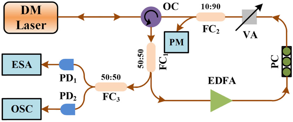
Fig. 1. Experimental setup. DM Laser, discrete-mode laser; OC, optical circulator; FC, fiber coupler; EDFA, erbium-doped fiber amplifier; PC, polarization controller; VA, variable optical attenuator; PM, power meter; PD, photodetector; ESA, electrical spectrum analyzer; OSC, oscilloscope.
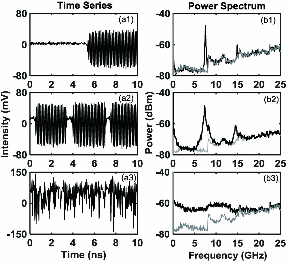
Fig. 2. Time series and power spectra of the ECF DM-SL output intensity when bias current is 40 mA, where the feedback ratio ξ f
Fig. 3. (a) Time series, (b) power spectra, and (c) phase portraits of the output of ECF DM-SL when I = 40 mA ξ f
Fig. 4. Duty cycle of the periodic oscillation as a function of ξ f I = 40 mA
Fig. 5. (a) Time series, (b) power spectra, and (c) phase portraits for the output of the DM-SL when I = 70 mA ξ f
Fig. 6. Mapping of dynamical states of the ECF DM-SL in the parameter space of ξ f I
Fig. 7. (a) Time series, (b) power spectra, and (c) phase portraits for the output of the DM-SL when τ = 20 ns J / J th = 3 κ 4.2 ns − 1 5.0 ns − 1
Fig. 8. Duty cycle of the periodic oscillation as functions of κ J / J th = 3 τ ext = 20 ns
Fig. 9. (a) Time series, (b) power spectra, and (c) phase portraits for the output of the DM-SL when τ = 20 ns J / J th = 6 κ = 7.9 ns − 1 κ = 9.3 ns − 1
Fig. 10. Dynamical state maps of the ECF DM-SL in the parameter space of normalized bias current and feedback strength when τ ext = 10 ns τ ext = 20 ns

Set citation alerts for the article
Please enter your email address
© Copyright 2018-2021 | Chinese Laser Press. All Rights Reserved 沪ICP备15018463号-20