Fig. 1. Sketch of the experimental arrangement. (a)–(c) Side view (from the y axis) of the gas jet (blue column), that exits the nozzle along the z axis. (d)–(f) Top view (from the z axis). The two synchronized, ns beams (red) propagate parallel to the y axis, on both sides (x axis) of the gas jet. The sudden laser heating of the plasma induces steep density fronts [(a) and (d)] that propagate out of the laser axis as blast waves [(b) and (e)]. The collision of two blast waves at the center of the gas jet [(c) and (f)] produces a sharp-gradient, thin, high-density plasma slab. Protons are accelerated from the interaction of the ps pulse with the plasma.

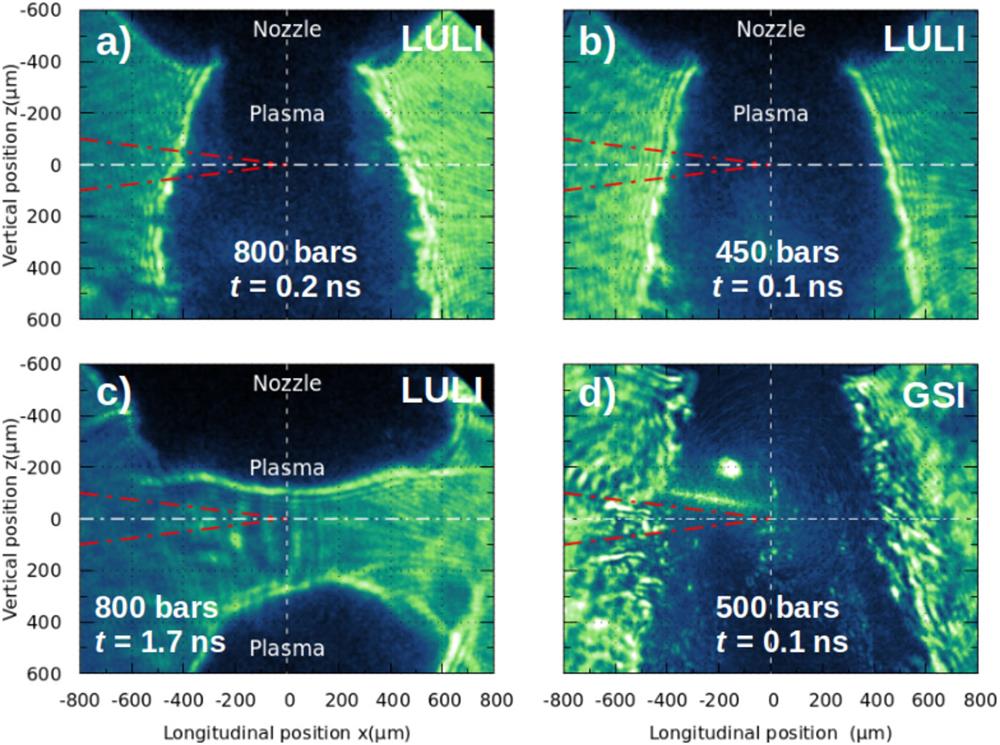
Fig. 2. Probe beam shadography from the plasma generated by the interaction of the ps beam with the high-density H₂ gas jet, at different backing pressures and different times from the ps-pulse arrival: (a)–(c) LULI experiment; (d) GSI experiment. At the top of each image (z < −400 μm) is the shadow of the nozzle. The ps beam propagates at z = 0 from left to right along the x axis (horizontal white dashed line), and is focused (red dashed lines) at the center of the jet (x = 0, y = 0). The vertical scale is the same for all four images.

Fig. 3. Time-resolved (streak camera) shadowgraphs along the ps-beam axis (x, at z = 0), for two gas jet pressures. The ps pulse arrives at t = 0 and propagates from left to right as in Fig. 2. The vertical scale is the same for both images.

Fig. 4. Proton spectra from the LULI experiment, without plasma tailoring, measured at 0°, 30°, and 70° from the ps-beam axis, for different gas jet backing pressures. The dashed lines are the noise levels of each spectrum. The laser-plasma parameters are the same as in Figs. 2 and 3. The vertical scale is the same for all three graphs.

Fig. 5. (a) Time-resolved [along the ps-beam axis (streak camera)] and (b) 2D space-resolved (GOI snapshot) shadowgraphs of the plasma tailored by one ns beam, at the entrance side of the ps beam, for a gas jet backing pressure of 200 bars. The dashed orange line highlights the croissant-like shape produced by the expansion of the HSW [see also Figs. 7(b), 8, and 10(a)]. The ns pulse propagates along the y axis (perpendicular to the image plane) and focuses at x = −300 μm, z = 0 (red circle). It arrives in the gas jet ∼2.7 ns before the ps pulse. The ps beam propagates at z = 0 from left to right along the x axis [horizontal white dashed line in (b)], and is focused [red dashed lines in (b)] at the center of the jet (x = 0, y = 0). The time integration window of the snapshot in (b) was ∼120 ps, centered on the ps-pulse arrival.

Fig. 6. Proton spectra from the LULI experiment, associated with the shadowgraphs of Fig. 5, for a plasma tailored at the entrance side of the ps beam. The vertical scale is the same for all three graphs.

Fig. 7. (a) Time-resolved [along the ps-beam axis (streak camera)] and (b) 2D space-resolved (GOI snapshot) shadowgraphs of the plasma tailored on the two opposite sides for a gas jet backing pressure of 200 bars. The energy in each ns beam is 4.5 J. The orange arrows in (a) indicates the minimum width of the shadowgraph (collision of the two HSWs). The horizontal line at t = 0 is the second-harmonic emission of the ps pulse along its propagation (x axis). The time integration window of the snapshot in (b) was ∼120 ps, ending just before the ps-pulse arrival. The blue dashed lines indicate the edges of the shadowgraph measured without plasma tailoring (Fig. 2).

Fig. 8. 2D space-resolved (GOI snapshot) shadowgraphs of the plasma tailored on the two opposite sides, for a gas jet backing pressure of 300 bars, at two different times: (a) before the collision of the HSWs; (b) just after their collision and the arrival of the ps pulse. The blue dashed lines indicate the edges of the shadowgraph measured without plasma tailoring (Fig. 2). The vertical scale is the same for both images.

Fig. 9. Proton spectra from four laser shots on the LULI experiment, in the case of a plasma tailored on both sides (as in Fig. 7), and a gas jet backing pressure of 300 bars on shot 1 and 200 bars on shots 2, 3, and 4. The dashed lines show the noise level of each spectrum. The vertical scale is the same for all three graphs.

Fig. 10. Typical result from the GSI experiment: (a) 2D space-resolved (GOI snapshot) shadowgraph of the plasma tailored on both sides; (b) associated proton spectrum measured at 50°. The gas jet backing pressure was 100 bars. The shadowgraph is 40 ps before the ps-pulse arrival.

Fig. 11. (a) Temporal evolution of the density profile along the ps-beam axis from 3D TROLL simulations. The two ns beams are focused 300 μm from both sides of the gas jet center. The initial maximum plasma density (at x = 0) is ne0=2×1020 cm⁻³ (=n_c/5). The spatial intensity profile of the ns beams is I(r) = 5.4 × 10¹⁴ exp[−(r/25)²], and the energy in each beam is 6 J. (b) Post-processing of the shadowgraphy diagnostic from the TROLL outputs. The cyan lineouts are density and shadowgraph profiles at t = 2.5 ns.

Fig. 12. Same as Fig. 11, but for a spatial profile of the ns beams with a low-intensity wing: I(r) = 3 × 10¹⁴{exp[−(r/25)²] + 0.0172 exp[−(r/110)²]} (W/cm²) and 4.5 J in each beam. The cyan lineouts are density and shadowgraph profiles at t = 2.3 ns.

Fig. 13. Spatial profiles of (a) the laser focal spot, (b) the electron temperature, (c) the electron density for the case without the wing in the intensity profile (left, Fig. 11) and with the wing (right, Fig. 12). (a) and (b) Are at 0.6 ns, the maximum of the laser, and (c) is at 2.3 ns (the time at which the HSWs collide in the case with the wing). The vertical scale is the same for all three images.

Table 1. Number of protons and total energy of the spectra for E_k > 1 MeV, measured at angles of 0°, 30°, and 70°, and for the different configurations of plasma tailoring. Obtained by integrating the spectra of Figs. 4, 6, and 9 between E_k = 1 and 3.5 MeV. Acceleration in the forward direction is highlighted in yellow.