Quantum fluctuation is the essential characteristic of quantum mechanics. Reducing quantum fluctuation below the standard fluctuation of zero-point level, called quantum squeezing, is always worth investigation [1], because quantum squeezing on the one hand plays an important role in fundamental physics, such as exploring the quantum-classical boundary [2–4], and on the other hand has an important value in practical applications, which include improving ultrasensitive detection [5–8] and enhancing coupling [9–11]. Squeezing of the mechanical mode is of special interest. The demonstration of mechanical squeezing was first reported in Ref. [12], using a spring constant tuned silicon microcantilever. With the development of quantum optics and the needs of precise quantum measurement, schemes realizing mechanical squeezing based on various systems, for instance the NV-center system [13] and trapped-ion system [14], have subsequently been proposed.

The cavity optomechanical system, due to the interaction between the cavity field and mechanical motion, provides us with a promising platform for high-precision measurements [15–18]. Therefore, the mechanical squeezing is necessary in the cavity optomechanical system in order to reduce additional noise [19–21]. The basic mechanism for generating mechanical squeezing is to introduce a mechanical parametric amplification in the cavity optomechanical system [22–25]. Using the mechanical parametric amplification, the squeezing of the mechanical oscillator has been achieved both theoretically and experimentally [26,27]. However, the squeezing can be restricted by the so called 3 dB limit due to the instability caused by the parametric amplification process [28–30]. To surpass the 3 dB limit of mechanical squeezing, schemes including injecting a squeezed light into the cavity [31,32], kicking the mechanical mode by the bang-bang control technique [33], jointing the effect between Duffing nonlinearity and parametric pump driving [34], and applying continuous weak measurement and feedback to the system [35] have been proposed. Recently, strong squeezing of the mechanical oscillator is demonstrated via the coherent feedback process, which can be performed by driving the cavity with two-tone driven field [36–40] or introducing a sine modulation of the free term to the mechanical oscillator in the optomechanical system [41].

On the other hand, quantum control is a powerful tool in modern quantum technologies [42–44]. In the Lyapunov control method, an index function (i.e., Lyapunov function) can monotonically increase or decrease to the target by designing the control field. Until now, Lyapunov control has been successfully used for processing diverse quantum tasks, such as realizing quantum synchronization [45], speeding up adiabatic passage [46], preparing quantum states [47], and designing quantum optical diode [48]. With the advances of microscale and nanoscale fabrication, it is becoming possible to engineer and to control the mechanical oscillator in the cavity optomechanical system. Recently, the mechanical oscillator with tunable frequency has been reported experimentally [49]. With the engineered mechanical oscillator, the quantum process, such as cooling [50] and squeezing [41], can be enhanced.

Although Lyapunov control and the optomechanical system have both been extensively studied separately, there are few studies which employ Lyapunov control to manipulate the optomechanical system. In this paper, by introducing a modulation of the frequency to the mechanical oscillator, a scheme to generate strong mechanical squeezing in an optomechanical system is proposed. Unlike modulating the frequency of the mechanical resonator periodically as in previous research [41,50,51], in our scheme, the frequency variations are designed based on Lyapunov control theory. By designing special time-varying mechanical frequency, the momentum variance of the mechanical mode can be decreased with time evolution, which results in the strong mechanical squeezing (larger than 10 dB in our parameter region). Moreover, the squeezing is immune to cavity decay in the weak coupling regime.

Our proposal generating mechanical squeezing based on Lyapunov control has three distinct merits. First, we can quickly obtain the strong squeezing, since the momentum variance of the mechanical oscillator decreases monotonically without oscillation. Second, our scheme generates squeezing without using assistant squeezing source. Therefore, the complexity of the experiment may be reduced. Third, as there is no parametric amplification term in our system, the instability caused by parametric amplification is avoided, thus leading to the squeezing beyond 3 dB possible.

The rest of this paper is organized as follows. We first briefly introduce the method of quantum Lyapunov control in Section 2. Then we present the model and its solution in Section 3. In Section 4, we discuss the generation of mechanical squeezing by employing the Lyapunov control. In Section 5, we give the proposal for detecting the obtained mechanical squeezing. The discussions and conclusions are summarized in Section 6.

We first briefly review quantum Lyapunov control method. For a controlled system, the total Hamiltonian can be generally expressed as H=Hres+∑nfn(t)Hn,(1)where Hn is the control Hamiltonian, and fn(t) is the time-varying control field with n=1,2,…. Hres is the rest Hamiltonian except the control Hamiltonian. The index function, which is also known as the Lyapunov control function, is selected according to the purpose. Here, we consider the mean value of operator O as the index function, i.e., V(t)=⟨O⟩=Tr(ρO). In the interaction picture, we have O˙=−i[O,Hres+∑nfn(t)Hn].(2)Therefore, the derivative of control function V(t) satisfies V˙(t)=Tr(ρO˙)=∑nfn(t)⟨−i[O,Hn]⟩,(3)where for simplicity, [O,Hres]=0 is assumed to obtain Eq. (3). Actually, even if [O,Hres]≠0, we can design one of the terms in the control field to cancel ⟨−i[O,Hres]⟩, hence we can always obtain the above equation. Supposing we want to reduce ⟨O⟩, we can design the control field as fn(t)=−c⟨−i[O,Hn]⟩* (c>0). The derivative of V(t) then becomes V˙(t)=⟨O˙⟩=−c∑n|⟨−i[O,Hn]⟩|2.(4)We see that V˙(t)≤0 is always satisfied, which means ⟨O⟩ will decrease monotonically during evolution. Therefore, the purpose of control has been realized by the selection of the control field fn(t)=−c⟨−i[O,Hn]⟩*. It should be noted that although fn(t) seems to depend on the evolution of ⟨−i[O,Hn]⟩*, we do not need to measure the value of ⟨−i[O,Hn]⟩*. The control field is actually obtained by the simulation, which is measurement-independent. In the experiment, one can pulse the simulated control field to the system, and the system will evolve toward the goal of design. In the following, we will decrease the momentum variance of the mechanical oscillator based on the Lyapunov control method, so as to obtain strong squeezing of the mechanical oscillator.

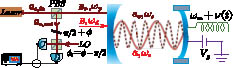
The system under consideration is a cavity optomechanical system, where a frequency-tunable mechanical oscillator couples to a single-mode cavity with the coupling strength g0, as schematically shown in Fig. 1. To tune the frequency of the mechanical resonator, one can apply a gate voltage Vg between the mechanical oscillator and the underlying electrode experimentally [52–54], or couple the mechanical oscillator with a low-Q driven assisted mode (see Appendix A for details). The Hamiltonian of the system then reads H=ℏωca†a+px22m+12mωr2(t)x2−ℏga†ax+iℏE(e−iωdta†−eiwdta),(5)where a (a†) is the annihilation (creation) operator of the cavity mode with the resonant frequency ωc, and x and px are the position and momentum operators of the mechanical resonator. Here ωr(t) is the controllable frequency of the mechanical mode tuned from the static frequency ωm and can be modulated by Vg. The last term in Eq. (5) describes the external classical driving to the cavity with the driven amplitude E and frequency ωd. By introducing the dimensionless position and momentum operators of the mechanical resonator (q,p) through q=mωmℏx,p=pxℏmωm,(6)the Hamiltonian of Eq. (5) can be rewritten as $$\begin{gathered} H=ℏωca†a+ℏωm2p2+ℏωr2(t)2ωmq2−ℏg0a†aq \\ +iℏE(e−iωdta†−eiwdta). \end{gathered}$$(7)

In the interaction picture with H0=ℏωda†a, and taking the dissipation and noise into consideration, we can write the quantum Langevin equations of the system as $$\begin{gathered} q˙=ωmp, \\ p˙=−ωr2(t)ωmq−γp+g0a†a+ξ, \\ a˙=−(κ+iΔc)a+ig0aq+E+2κain, \end{gathered}$$(8)where Δc=ωc−ωd is the detuning between the cavity mode and driven field, and κ and γ represent the damping rates of the optical mode and mechanical mode, respectively. The noise operators ain and ξ satisfy the following correlation functions: $$\begin{gathered} ⟨ain(t)ain†(t′)⟩=(n¯cT+1)δ(t−t′), \\ ⟨ξ(t)ξ(t′)+ξ(t′)ξ(t)⟩/2=γ(2n¯mT+1)δ(t−t′), \end{gathered}$$(9)under Markovian approximation, where n¯cT and n¯mT are the equilibrium mean thermal photon numbers of the cavity mode and mechanical oscillator, respectively. Generally, n¯cT≈0 due to the high optical frequency.

By performing the standard linearization process, we write the operators as their mean values plus small quantum fluctuations, i.e., a=α+δa, q=qc+δq, p=pc+δp, where α, qc, and pc are complex numbers determined by $$\begin{gathered} q˙c=ωmpc, \\ p˙c=−ωr2(t)ωmqc−γpc+g0|α|2, \\ α˙=−(κ+iΔc′)α+E, \end{gathered}$$(10)with Δc′=Δc−g0qc. Correspondingly, the fluctuation parts satisfy $$\begin{gathered} δ˙q=ωmδp, \\ δ˙p=−ωr2(t)ωmδq−γδp+G(δa†+δa)+ξ, \\ δ˙a=−(κ+iΔc′)δa+iGδq+2κain, \end{gathered}$$(11)where G=g0α is the effective coupling rate. It should be pointed out that G can achieve any desirable value in principle by modulating the corresponding driving E(t) [55,56]. By introducing the quadrature operators δX=(δa+δa†)/2, δY=(δa−δa†)/2i and the corresponding noise operators Xin=(ain+ain†)/2, Yin=(ain−ain†)/2i, the linearized Langevin equations for the fluctuation operators can be concisely expressed as u˙(t)=A(t)u(t)+N(t),(12)where u(t)=(δX(t),δY(t),δq(t),δp(t))T, N(t)=(2κXin(t),2κYin(t),0,ξ(t))T, and A(t) is A(t)=(−κΔc′00−Δc′−κ2G0000ωm2G0−ωr2(t)/ωm−γ).(13)The formal solution of Eq. (12) can then be given as u(t)=L(t)u(0)+L(t)∫0tdτ′L−1(τ′)N(τ′),(14)where L(t)=Texp[∫0tdτA(τ)]L(0) with T the time order operator.

To calculate the quantum fluctuation of the mechanical mode, we introduce the covariance matrix R(t) defined as Rij(t)=[⟨ui(t)uj(t)+uj(t)ui(t)⟩]/2.(15)By using Eqs. (14) and (15), we can obtain R=L(t)R(0)LT(t)+L(t)M(t)LT(t),(16)where $$\begin{gathered} M(t)=12[W(t)+WT(t)], \\ W(t)=∫0tdτ∫0tdτ′L−1(τ′)C(τ,τ′)[L−1(τ)]T. \end{gathered}$$(17)Here C(τ,τ′) is the noise operator correlation matrix with its matrix element Cij(τ,τ′)=⟨Ni(τ)Nj(τ′)⟩. Obviously ⟨Nij(τ)Nij(τ′)+NijT(τ)NijT(τ′)⟩/2=Dijδ(τ−τ′).(18)Here, Dij is the matrix element of the diagonal matrix D=Diag[κ,κ,0,γ(2n¯mT+1)]. Substituting Eq. (18) into Eq. (17), we obtain M(t)=∫0tdτL−1(τ)D(τ)[L−1(τ)]T.(19)By substituting Eq. (19) into Eq. (16), the derivative of the covariance matrix is given by R˙(t)=A(t)R(t)+R(t)AT(t)+D.(20)

For a mechanical oscillator, the rotating quadrature operator is X(θ,t)=cosθ·δq+sinθ·δp. Correspondingly, the variance of the mechanical quadrature operator ΔX2=⟨X2(θ,t)⟩−⟨X(θ,t)⟩2 is given by $$\begin{gathered} ΔX2=cos2θ⟨δq2⟩+sin2θ⟨δp2⟩+12sin2θ(⟨δqδp⟩+⟨δpδq⟩) \\ =cos2θR33+sin2θR44+12sin2θ(R34+R43). \end{gathered}$$(21)Therefore the variance of the quadrature operator X(θ,t) for the mechanical mode can be obtained by solving Eq. (20) with the initial condition R(0)=Diag[1/2,1/2,1/2,1/2]. Here the initial fluctuation 1/2 means the cavity and mechanical fields are both in vacuum states, which can be realized by respectively precooling the cavity mode and mechanical resonator to their ground states.

Now we employ the Lyapunov control method introduced in Section 2 to generate the mechanical quadrature squeezing. The index ΔX2 is selected as the Lyapunov function V(t), i.e., V(t)=ΔX2. Obviously, V(t)>0. And the time derivative of V(t) by using Eq. (21) is calculated as V˙(t)=cos2θR˙33+sin2θR˙44+12sin2θ(R˙34+R˙43),(22)where $$\begin{gathered} R˙33=ωm(R34+R43), \\ R˙44=−2γR44−ωr(t)2ωm(R34+R43) \\ +2G(R14+R41)+γ(2n¯mT+1), \\ R˙34=ωmR44−ωr(t)2ωmR33−γR34+2GR31, \\ R˙43=ωmR44−ωr(t)2ωmR33−γR43+2GR13. \end{gathered}$$(23)

In our model, ωr(t) is adjustable, and therefore we can select ωr(t) as a control field. However, only the static frequency ωm appears in the first equation of Eq. (23), thus the first term of Eq. (22) is not controllable. Therefore, we can set θ=π/2 to cancel the first term of Eq. (22) for simplicity. In this case, the Lyapunov function V(t)=Δp2 is the variance of momentum operator. Then the time derivative of V(t) becomes $$\begin{gathered} V˙(t)=−2γR44−ωr2(t)ωm(R34+R43)+2G(R14+R41) \\ +γ(2n¯mT+1). \end{gathered}$$(24)In the right-hand side of the above equation, the first term −γR44<0 is always satisfied. And if we choose the control field ωr2(t)=cωm(R34+R43) with c>0, the second term −ωr2(t)ωm(R34+R43)=−c|R34+R43|2≤0. In principle, we can choose G=−c2(R14+R41) with c2>0 to guarantee the third term 2G(R14+R41)≤0. However this setting is not necessary, because the correlation between the cavity field and mechanical oscillator R14 and R41 is small. At the weak coupling case, the effect of the third term can be neglected. For high quality factor mechanical oscillator and low bath temperature, the last term γ(2n¯mT+1) contributes small to the equation of derivative of V. For the convenience of analysis, we ignore the influence of the last two terms. And in the numerical simulations, we do not use this approximation. If ignoring the last two terms, V˙(t)≈−2γR44−c|R34+R43|2,(25)with ωr2(t)=cωm(R34+R43).(26)It is obvious that V˙(t) is always less than or equal to zero, which means the index function V(t)=Δp2 will decrease monotonically during evolution, and may approach 0 with ωr2(t)=cωm(R34+R43). Therefore, the momentum variance of mechanical oscillator Δp2 can be reduced to below the zero-point level, as a result the squeezed mechanical oscillator is obtained. We should note that although ωr2(t)=cωm(R34+R43) is dependent of R34+R43, the experimental detection of R34+R43 is not necessary, and the control field ωr2(t) is obtained by simulation. This is an open-loop control scheme, which uses the closed-loop idea to solve the problem of open-loop control.

To examine the above analysis, we need to simulate the dynamics of the system. In Fig. 2(a), the momentum variance of mechanical oscillator Δp2 depending on time at G=0.1ωm is plotted, in which case the time-varying frequency of the mechanical oscillator is shown in Fig. 2(c). It is obvious that Δp2 decreases monotonically with time evolution as shown by the solid blue line, which agrees with the above discussions. Without control, we see that Δp2 oscillates near the zero-point level 0.5. However, with the Lyapunov control, Δp2 will be lower than 0.1, and thus we realize strong squeezing of the mechanical oscillator. The evolution of momentum variance Δp2 at G=0.5ωm is shown in Fig. 2(b). Correspondingly, in Fig. 2(d), we give the time-dependent mechanical frequency for the control case. With this higher coupling strength, we see that Δp2 is still oscillating around 0.5 without control. Although Δp2 does not always decrease with respect to time t with the Lyapunov control, the stable Δp2 is about 0.355, which means we can still realize squeezing at G=0.5ωm.

In Figs. 3(a) and 3(b), we further study the control effect of the control field described by Eq. (26) under different G and Δc′, while Figs. 3(c) and 3(d) are the control fields. It is seen that the larger G is, the less monotonic Δp2 is. This is resonant because Eq. (25) is obtained in the approximation by neglecting the effect of 2G(R14+R41) as described in Eq. (24), and this approximation is only valid for the weak coupling case. For ultrastrong coupling G, Δp2 will oscillate with time evolution and the squeezing will disappear; therefore, the above Lyapunov control scheme is valid for the weak coupling case. In principle, the squeezing is best with G=0, while squeezing in the cavity optomechanical system is of significance, so we discuss the squeezing with G≠0. In Fig. 3(b), it is obvious that the above Lyapunov control scheme works well for the sideband regime, especially for the red sideband case. Generally speaking, the red sideband condition Δc′=ωm is used for the ultrasensitive detection; therefore, the squeezing generated by our scheme may be useful for enhancing ultrasensitive detection.

In order to clearly see the squeezing intuitively, we present the Wigner function of mechanical oscillator Wm in Fig. 4. It is obvious that Wm has the same distribution on q and p at ωmt=0; hence, there exists no squeezing at the initial time. With the time evolution, when ωmt=30, the mechanical quadrature p is obviously squeezed, and the maximum squeezed direction is along the position p.

To further study the robustness of our scheme, we now simulate the squeezing level S as a function of time t with different cavity decay κ and thermal phonon number n¯mT, where the squeezing level S in the decibel unit is defined by S=−10log10(Δp2/Δpzp2).(27)Here Δpzp2=0.5 is the standard fluctuation in the zero-point level.

Figure 5(a) shows that the proposed scheme is affected little by the cavity decay κ. When the system changes from the resolved sideband regime to the unresolved sideband regime, the squeezing level S decreases a little. This is reasonable since the cavity field has little effect on the proposal in the weak coupling regime as discussed above. Hence our scheme is robust to cavity decay. Moreover, the squeezing level can surpass 3 dB limit at a fast time, which suggests that the strong squeezing of the mechanical oscillator can be attained quickly even at large cavity decay. From Fig. 5(b), we see that the squeezing level S decreases a lot when the thermal phonon number n¯mT increases from 10 to 104. This can be understood by Eq. (24). With large n¯mT, the term γ(2n¯mT+1) contributes to the derivative of V, and the approximation equation shown by Eq. (25) is not valid. Therefore, Δp2 will not decrease monotonically with time evolution, which leads to the squeezing level S decreasing with large n¯mT. Nevertheless, we can get relatively large squeezing over a long period of time when the thermal phonon number n¯mT is not very large. For the thermal phonon number larger than 103, one should employ other methods to reduce the temperature of the bath before using Lyapunov control.

Finally, we discuss the detection of the generated mechanical squeezing in our scheme. As depicted in Fig. 1, an ancillary cavity mode as with frequency ωs is introduced to the system for detection. Meanwhile, the ancillary mode as is driven by a weak pump field with amplitude Ep and frequency ωp. The total Hamiltonian with the ancillary mode included is Ht=H+ℏωsas†as−ℏgsas†asq+iℏEp(e−iωptas†−h.c.),(28)where H is given by Eq. (7), and gs is the coupling strength between the ancillary mode as and the mechanical oscillator. The pump field of as is selected to be very weak so that the ancillary mode reaches a small steady-state amplitude αs, i.e., αs≪α, thus Gs≪G. Therefore, we can safely neglect the backaction of as on the mechanical oscillator, and the dynamics of mechanical mode δq (δp) and cavity mode δX (δY) can still be well described by Eq. (12). We will discuss the correction later. Now we describe the detection of the squeezing. With the dissipation κs and noise as,in taken into consideration, the linearized equation for the ancillary mode as is δ˙as=−(κs+iΔs′)δas+iGsδq+2κsas,in,(29)where Δs′ is the effective detuning. If we choose parameters so that Δs′=ωm≫Gs/2, κs, by neglecting the terms rapidly oscillating at the frequency 2ωm, the above equation can be rewritten as δ˙as=−(κs+iΔs′)δas+iGs2δb+2κsas,in,(30)where δb=(iδp+δq)/2. Under κs≫Gs/2, the ancillary mode δas will adiabatically follow the dynamics of δb [57], and is given by δas=iGs2(κs+iΔs′)δb+2κsκs+iΔs′as,in.(31)Using the input–output relation δas,out=2κsδas−δas,in, we have δas,out=iκsGsκs+iΔs′δb+(2κsκs+iΔs′−1)as,in.(32)The above equation shows that the output field of the ancillary mode gives a direct measurement of the mechanical oscillator. This method has been proposed to detect the entanglement between the cavity field and mechanical oscillator [58]. Here we use it to measure the momentum variance of the mechanical oscillator. By defining the quadrature operator δXs,out(ϕ)=(δas,oute−iϕ+δas,out†eiϕ)/2, one can obtain $$\begin{gathered} δXs,out(ϕ)=Gsκs(Δs′cosϕ+κssinϕ)Δs′2+κs2δq \\ +Gsκs(Δs′sinϕ−κscosϕ)Δs′2+κs2δp+Fad, \end{gathered}$$(33)where Fad is the noise term. By choosing appropriate ϕ such that tanϕ=−Δs′/κs, the term that contains δq is removed, and we can obtain δXs,out(ϕ)=Gsκs(Δs′sinϕ−κscosϕ)Δs′2+κs2δp+Fad.(34)

It is obvious that δp can be directly reflected in δXs,out(ϕ). Therefore, we can detect the generated squeezing of the mechanical mode by measuring the variance of the output ancillary mode δXs,out(ϕ). However, it should be recognized from Eq. (34) that δXs,out(ϕ) is a weak signal. In order to amplify the signal, the balanced homodyne detection method is used here, where the local oscillator (LO) noise is simultaneously eliminated. As illustrated in Fig. 1, the signal field δas,out first passes through a phase shifter to rotate a phase π/2+ϕ, where π/2 is used to compensate for the phase shift between the reflected and incident field in the polarizing beam splitter (PBS), and ϕ is used to rotate the field δas,out by a phase ϕ so as to detect the momentum variance of the mechanical oscillator. Then the rotated field δas,out is superimposed with a strong LO through a 50/50 beam splitter, in which the output signal is ncd=−i(|βl|e−iϕlδas,out†−|βl|eiϕlδas,out),(35)where |βl| and ϕl are respectively the amplitude and phase of LO. Therefore, the variance of the output signal is (Δncd)2=4|βl|2ΔXs,out2(ϕl+π/2),(36)where ΔXs,out2(ϕ)=⟨δXs,out2(ϕ)⟩−⟨δXs,out(ϕ)⟩2. From the above equation, we see that the weak signal ΔXs,out2(ϕl+π/2) is amplified in the detection by an amplification factor 4|βl|2. By substituting Eq. (34) into Eq. (36), and setting the phase of the LO ϕl=π/2−ϕ, we can get the relationship between the oscillator variance Δp2 and (Δncd)2; therefore, the generated mechanical squeezing can be detected by the proposal discussed above.

It should be noted that the backaction of as on the mechanical oscillator is neglected in the detection proposal. Whether the added ancillary mode as can affect the dynamics of the mechanical oscillator or not should be verified. Therefore, it is necessary to compare the dynamics of the mechanical oscillator with and without the ancillary mode. By taking the system with the ancillary detection mode as into consideration, the dynamics equation of the 6×6 covariance matrix R′ satisfies R˙′(t)=A′(t)R′(t)+R′(t)A′T(t)+D′,(37)where D′=Diag[κ,κ,0,γ(2n¯mT+1),κs,κs], and A′(t)=(−kΔc′0000−Δc′−κ2G000000ωm002G0−ωr2(t)ωm−γ2Gs00000−κsΔs′002Gs0−Δs′−κs).(38)

To examine the influence on the system of the ancillary detection mode, we present the time evolution of Δq2 with and without the detection mode together in Fig. 6, where the control field designed in Fig. 2(c) is used for both of the two cases. The result shows that the evolution of Δq2 agrees very well for the two cases. Therefore, we can safely neglect the backaction of as on the mechanical oscillator.

We now discuss the experimental feasibility of our scheme. For the cavity optomechanical system, κ/ωm=10−2–10 and γ/ωm=10−9–10 have been reported in experiments (see Table II in Ref. [59]). Obviously the parameters κ/ωm=0.1, γ/ωm=10−6 used in our simulations are within the current experiments. From Fig. 2, we know that the squeezing process is fast, and hence we can assume that n¯mT is not affected by the tuning frequency ν(t) but only determined by the static frequency ωm; therefore, the thermal phonon number is evaluated by n¯mT=[exp(ℏωm/kBT)−1]−1. Moreover, if the frequency of the mechanical oscillator is tuned by the method described in Appendix A, the thermal phonon number of the mechanical oscillator n¯m is just determined by the frequency of the mechanical oscillator ωm after ignoring the vacuum noise from the ancillary cavity. In Fig. 5(b), the thermal phonon numbers n¯mT=10, 103, and 104 are corresponding to the temperature of the bath T=0.01K, 0.9 K, and 9.6 K, respectively, when frequency of the mechanical oscillator is ωm/2π=20MHz. Currently, the temperature of thermal bath T=10mK has been reported experimentally, and thus the proposed scheme is achievable within the current experiments.

In addition, the frequency-tunable mechanical oscillator has been realized experimentally [52–54], and we also give an alternative method to tune the mechanical frequency in Appendix A, which is experimentally feasible. For many proposals realizing mechanical squeezing, the squeezing level is limited by the 3 dB limit due to the unsteadiness of the system caused by the parametric amplification process. However, in our scheme, the frequency of the mechanical oscillator is time-dependent and is designed by the Lyapunov control method, which can guarantee that the fluctuation of the mechanical mode always decreases with time evolution without divergence [see the evolution of Δq2 in Figs. 2(a) and 2(b)]. Therefore, the system can be stable with the squeezing level beyond 3 dB.

To conclude, in this paper, by using the Lyapunov control method, we have presented a scheme for generating mechanical squeezing. By designing the time-varying mechanical frequency, the momentum variance of the mechanical mode can decrease with the time evolution under the weak coupling case. As a consequence, the squeezing exceeding the 3 dB limit is obtained quickly, and the largest squeezing can be larger than 10 dB. In addition, the squeezing is robust against cavity decay for the weak coupling regime. In the strong coupling case, the obtained squeezing is not as good as the weak coupling case due to the backaction. Although the mechanical thermal phonon number can destroy the preparation of mechanical squeezing, we can obtain strong squeezing at the temperature within the current experiment technology. In addition, we discuss the detection of the momentum variance Δp2 by introducing an ancillary mode. Via homodyne detection, we simulate Δp2 with and without an ancillary mode. The results show that the backaction of the ancillary mode can be ignored, which ensures the validity of the detection protocol. Our scheme provides a potential way for realizing squeezing of the mechanical motion beyond 3 dB.

Acknowledgment. We would like to thank Mr. Ye-Xiong Zeng, Cheng-Hua Bai and Ming-Hui Du for helpful discussions. Many thanks to Prof. Ying Gu for constructive suggestions.