• Photonics Research
  • Vol. 9, Issue 7, 1310 (2021)
Zarko Sakotic1、*, Alex Krasnok2, Andrea Alú2、3, and Nikolina Jankovic1
Author Affiliations
  • 1BioSense Institute-Research Institute for Information Technologies in Biosystems, University of Novi Sad, Dr Zorana Djindjica 1a, 21101, Novi Sad, Serbia
  • 2Advanced Science Research Center, City University of New York, New York, New York 10031, USA
  • 3Physics Program, Graduate Center, City University of New York, New York, New York 10016, USA
  • show less
    DOI: 10.1364/PRJ.424247 Cite this Article Set citation alerts
    Zarko Sakotic, Alex Krasnok, Andrea Alú, Nikolina Jankovic. Topological scattering singularities and embedded eigenstates for polarization control and sensing applications[J]. Photonics Research, 2021, 9(7): 1310 Copy Citation Text show less
    (a) Sketch of a PEC-backed slab with Drude dispersion; bulk mode dispersion for TM-polarized light. At kx=ky=0 and ωp the system supports a symmetry-protected EE, as indicated by the Q-factor divergence on the right. (b) Dispersion of scattering matrix singularities in the imaginary frequency space—zeros (perfectly absorbing states) and poles (eigenmodes). Lossy or gainy Drude model enables the creation of a ring of perfect absorption/lasing points at the real frequency axis. (c) Vector flow of the complex reflection coefficient rTM in the wavenumber–frequency plane. The EE splits into two vortices—a saddle point and a source point—which move away from each other as loss increases.
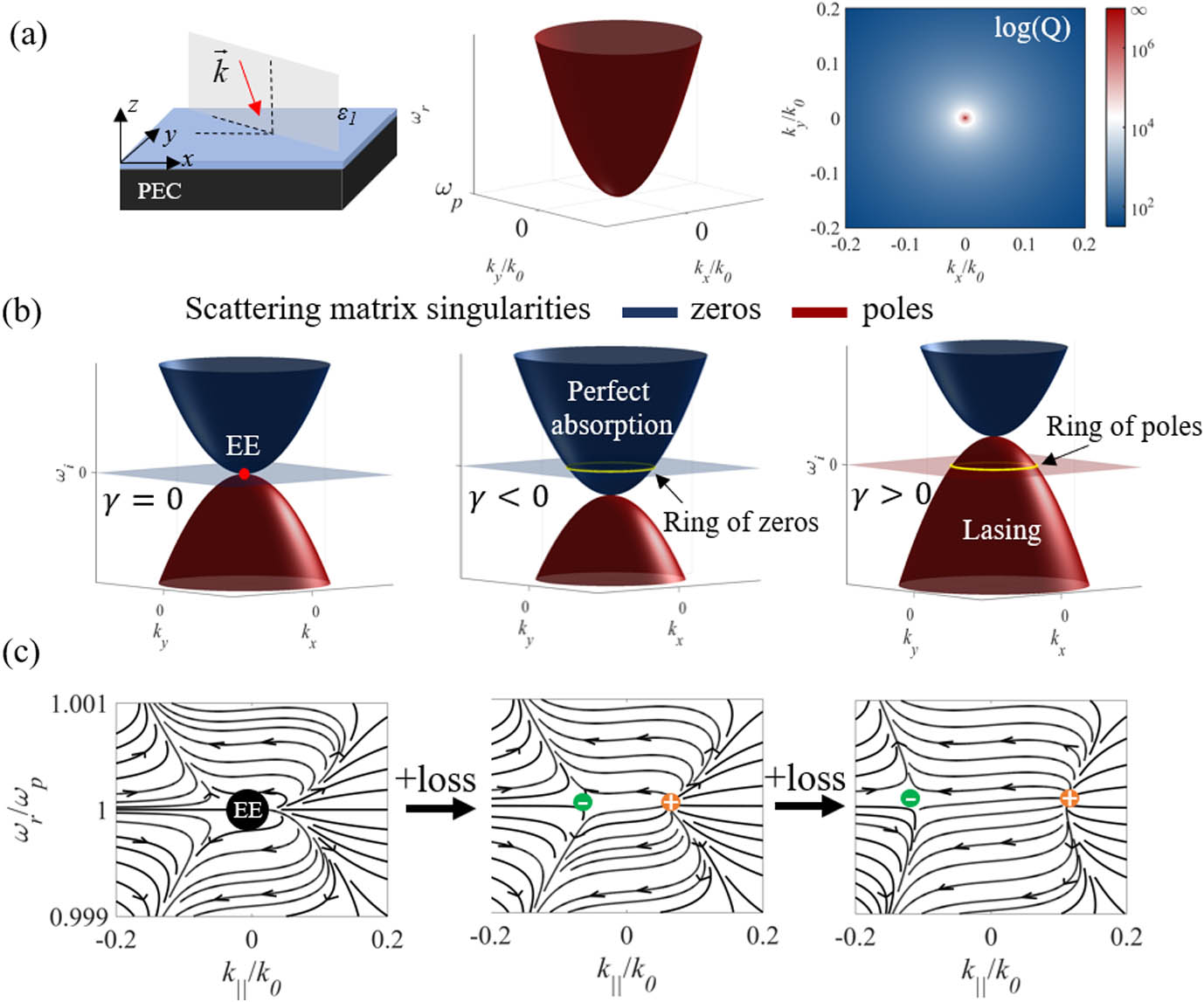
    Fig. 1. (a) Sketch of a PEC-backed slab with Drude dispersion; bulk mode dispersion for TM-polarized light. At kx=ky=0 and ωp the system supports a symmetry-protected EE, as indicated by the Q-factor divergence on the right. (b) Dispersion of scattering matrix singularities in the imaginary frequency space—zeros (perfectly absorbing states) and poles (eigenmodes). Lossy or gainy Drude model enables the creation of a ring of perfect absorption/lasing points at the real frequency axis. (c) Vector flow of the complex reflection coefficient rTM in the wavenumber–frequency plane. The EE splits into two vortices—a saddle point and a source point—which move away from each other as loss increases.
    (a) Sketch of the planar multilayer structure under oblique illumination. (b) Permittivity dispersion of the top layer. (c), (d) Reflection-zero dispersion in the ENZ and ENP regions. For the ENZ case, thicknesses were chosen as t/λENZ=0.05 and d=λENZ/4, and for the ENP case t/λENZ=0.007 and d=λ0/2. Dielectric permittivity is εd=1. (f)–(h) Phase and amplitude plots of TM reflection in the lossless and lossy cases for ENZ EEs. (i)–(k) Phase and amplitude of TM reflection in the lossless and lossy cases for ENP EEs. (l)–(n) Phase and amplitude of TE reflection in the lossless and lossy cases for ENP EEs.
    Fig. 2. (a) Sketch of the planar multilayer structure under oblique illumination. (b) Permittivity dispersion of the top layer. (c), (d) Reflection-zero dispersion in the ENZ and ENP regions. For the ENZ case, thicknesses were chosen as t/λENZ=0.05 and d=λENZ/4, and for the ENP case t/λENZ=0.007 and d=λ0/2. Dielectric permittivity is εd=1. (f)–(h) Phase and amplitude plots of TM reflection in the lossless and lossy cases for ENZ EEs. (i)–(k) Phase and amplitude of TM reflection in the lossless and lossy cases for ENP EEs. (l)–(n) Phase and amplitude of TE reflection in the lossless and lossy cases for ENP EEs.
    Charge annihilation for the lossy structures (γ=0.003ωp) considered in Fig. 2. (a) Phase of reflection for the ENZ case. Two charges annihilated and one remaining. (b) The reflection-zeros associated with these charges have vanished. (c) Same as (a) for the ENP case. (d) Same as (b) for the ENP case.
    Fig. 3. Charge annihilation for the lossy structures (γ=0.003ωp) considered in Fig. 2. (a) Phase of reflection for the ENZ case. Two charges annihilated and one remaining. (b) The reflection-zeros associated with these charges have vanished. (c) Same as (a) for the ENP case. (d) Same as (b) for the ENP case.
    Polarization manipulation. (a) Ellipsometric parameter ψ=arctan⁡(rTM/rTE) normalized to π. (b) Total reflectance as an efficiency indicator. (c) Polarization ellipses in the output for CP input. Red and black colors indicate handedness (red for RCP, black for LCP). (d) Polarization ellipses in the output for 45° LP input.
    Fig. 4. Polarization manipulation. (a) Ellipsometric parameter ψ=arctan(rTM/rTE) normalized to π. (b) Total reflectance as an efficiency indicator. (c) Polarization ellipses in the output for CP input. Red and black colors indicate handedness (red for RCP, black for LCP). (d) Polarization ellipses in the output for 45° LP input.
    (a) Sensing scheme based on phase singularities. (b) Phase of the reflection coefficient as the frequency is changed and passes near the vortex. Inset: |rTM| near the EE at 50°; phase sensitivity to small changes of the gap permittivity. (c) Sensitivity for three different configurations; improvement due to enhanced Q factor with antireflection coating and DBR.
    Fig. 5. (a) Sensing scheme based on phase singularities. (b) Phase of the reflection coefficient as the frequency is changed and passes near the vortex. Inset: |rTM| near the EE at 50°; phase sensitivity to small changes of the gap permittivity. (c) Sensitivity for three different configurations; improvement due to enhanced Q factor with antireflection coating and DBR.
    Sensitivity of the reflection coefficient and sensitivity for different incidence angles. (a) The reflection coefficient of the DBR structure in Fig. 5(c) is extremely sensitive to small changes in incidence angle, resulting in 1 order of magnitude change in sensitivity for extremely small angle changes. (b)–(d) Near annihilation point sensing with stabilized sensitivity. The amplitude of the reflection coefficient is more robust to incidence angle variations, with the sensitivity not changing substantially for 1° changes in angle for (b) and (c), and 0.2° for (d).
    Fig. 6. Sensitivity of the reflection coefficient and sensitivity for different incidence angles. (a) The reflection coefficient of the DBR structure in Fig. 5(c) is extremely sensitive to small changes in incidence angle, resulting in 1 order of magnitude change in sensitivity for extremely small angle changes. (b)–(d) Near annihilation point sensing with stabilized sensitivity. The amplitude of the reflection coefficient is more robust to incidence angle variations, with the sensitivity not changing substantially for 1° changes in angle for (b) and (c), and 0.2° for (d).
    Transmission line model for (a) single slab and (b) spacer structure.
    Fig. 7. Transmission line model for (a) single slab and (b) spacer structure.
    Annihilation of charges in a system with multiple embedded eigenstates. Reflection coefficient amplitude (left) and phase (right).
    Fig. 8. Annihilation of charges in a system with multiple embedded eigenstates. Reflection coefficient amplitude (left) and phase (right).
    Annihilation of charges in a system with multiple embedded eigenstates.
    Fig. 9. Annihilation of charges in a system with multiple embedded eigenstates.
    ENP scattering features. (a) For t=200 nm, propagating modes in the top layer are visible in the lossless case, along with the spacer mode. (b) Phase vortices appear in the lossy case; top layer modes are strongly suppressed and not visible. (c) Perfect absorption points appear in the lossy case. (d)–(f) Same as (a)–(c) for t=40 nm.
    Fig. 10. ENP scattering features. (a) For t=200  nm, propagating modes in the top layer are visible in the lossless case, along with the spacer mode. (b) Phase vortices appear in the lossy case; top layer modes are strongly suppressed and not visible. (c) Perfect absorption points appear in the lossy case. (d)–(f) Same as (a)–(c) for t=40  nm.
    (a) Sketch of the polarization plane and the reflection problem under analysis. (b) Ellipsometric parameter ψ=arctan⁡(rTM/rTE) where zeros of different polarizations are highlighted. Output polarization dependence on the material loss parameter γ (c) for CP input at TM zero, (d) 45° LP input at TM zero, (e) CP input at TE zero, and (f) 45° LP input at TE zero.
    Fig. 11. (a) Sketch of the polarization plane and the reflection problem under analysis. (b) Ellipsometric parameter ψ=arctan(rTM/rTE) where zeros of different polarizations are highlighted. Output polarization dependence on the material loss parameter γ (c) for CP input at TM zero, (d) 45° LP input at TM zero, (e) CP input at TE zero, and (f) 45° LP input at TE zero.
    (a) TE reflection coefficient dispersion for the incident angle where charges appear. Inset shows the structure under consideration and an illustration of the position of charges for different backing materials. (b) Analytical and numerical reflectance for the realistic model (shown in the inset) around ωTO.
    Fig. 12. (a) TE reflection coefficient dispersion for the incident angle where charges appear. Inset shows the structure under consideration and an illustration of the position of charges for different backing materials. (b) Analytical and numerical reflectance for the realistic model (shown in the inset) around ωTO.
    Zarko Sakotic, Alex Krasnok, Andrea Alú, Nikolina Jankovic. Topological scattering singularities and embedded eigenstates for polarization control and sensing applications[J]. Photonics Research, 2021, 9(7): 1310
    Download Citation