
Yunquan Liu, Meng Han. Recent Research Advances in Strong-Field Atomic Tunneling Ionization[J]. Acta Optica Sinica, 2021, 41(1): 0102001
- Acta Optica Sinica
- Vol. 41, Issue 1, 0102001 (2021)
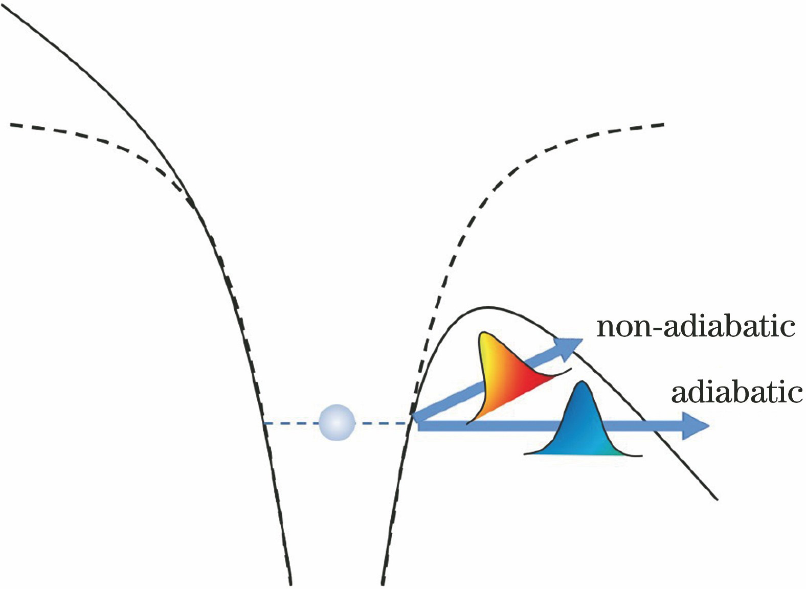
Fig. 1. Physical picture of tunneling ionization. Horizontal channel represents adiabatic tunneling, and upwards tilted channel represents non-adiabatic tunneling
![Spatial distributions of the tunneling exit of electron wave packets[26]. (a) Distribution of the tunneling exit of electron wave packets along the z axis; (b) distribution of the tunneling exit of electron wave packets along the x axis; (c) absolute distance distribution of the tunneling exit of electron wave packets. The red line shows the laser field in corresponding direction, the violet dashed line and the black line depict the](/richHtml/gxxb/2021/41/1/0102001/img_2.jpg)
Fig. 2. Spatial distributions of the tunneling exit of electron wave packets[26]. (a) Distribution of the tunneling exit of electron wave packets along the z axis; (b) distribution of the tunneling exit of electron wave packets along the x axis; (c) absolute distance distribution of the tunneling exit of electron wave packets. The red line shows the laser field in corresponding direction, the violet dashed line and the black line depict the
Fig. 3. Initial momentum distributions of tunneling electron wave packets[26]. (a) Initial transverse momentum distributions of electron wave packets; (b) initial longitudinal momentum distributions of electron wave packets; (c) transverse (dashed line) and longitudinal (solid line) momentum distributions when t=0.05T, 0.10T, and 0.15T; (d) initial transverse (solid line) and longitudinal (dashed line) momentum distributions a
Fig. 4. Photoelectron momentum distributions of final state in polarization plane[26]. (a) TDSE model; (b) parabolic coordinate tunneling model; (c) TIPIS model
Fig. 5. Measured photoelectron momentum spectra in orthogonal polarization two-color fields with comparable intensities[33]. Numbers in right-upper corner represent the relative phase
Fig. 6. Two-color light fields with comparable intensities and electron interference dynamics at the relative phase of 0.5π[33]. (a) Temporal sketch of the light field. The black line, red line, and blue line indicate the synthesized electric field versus time, negative vector potentials of 800 nm light, and negative vector potentials of 400 nm light, respectively; (b) spatial view of the light field. The deepening of yellow arrows represents the increas
Fig. 7. Simulated electron momentum distributions at relative phase of 0.5π[33]. (a) Result calculated by CCSFA model without plain sub-barrier phase; (b) result calculated by CCSFA model with plain sub-barrier phase; (c) result obtained by solving SFA model; (d) result obtained by solving TDSE model; (e) angular distributions of first-order ATI obtained by experiment and CCSFA model
Fig. 8. Mechanism of producing spatially separated spin polarization photoelectrons using OTC light field at relative phase of zero[45]. (a) Illustrations of OTC light field and circular orbitals;(b) synthesized laser electric field. During a half of laser cycle, electric field is clockwise rotating along the path of A-B-C, and in another half cycle, electric field is anticlockwise rotating along the path of C-B-A;(c) distribution of CG coefficients. Fro
Fig. 9. Results calculated by orbital-resolved SFA model[45]. Calculated photoelectron subcycle momentum distributions of (a) p- and (b) p+ orbitals of 2P1/2, respectively; (c) asymmetry of momentum-resolved normalized yield
Fig. 10. Time-resolved spin-polarization dynamics[45]. (a) Synthesized electric field and yield of electron wave packets at laser crests of A-C; (b) instantaneous angular velocity of light polarization vector; (c) instantaneous spin-polarization degree of 2P1/2 and 2P3/2 ionic states; (d) instantaneous normalized yield asymmetry of 2P1/2 and 2P3/2 ionic states

Set citation alerts for the article
Please enter your email address
© Copyright 2018-2021 | Chinese Laser Press. All Rights Reserved 沪ICP备15018463号-20