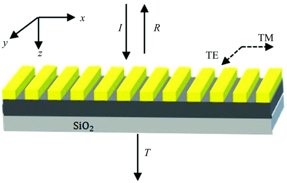
Fig. 1. One via wavelength grating structure diagram

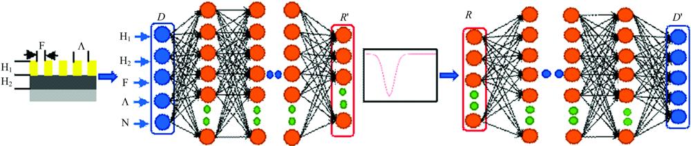
Fig. 2. Neural network structure
(a): Forward simulation network; (b): Reverse-design network

Fig. 3. (a) Forward simulation Loss function curve; (b) Inverse design Loss function curve

Fig. 4. Series neural network
R: Expected spectral response; R': Forward simulation prediction spectrum; D: Sample structure of the original training set; D': Reverse design forecast structure. The red frame is the forward simulation network. The Loss function is modified to solve the problem that the network cannot be fitted due to the non-uniqueness of the data. The middle layer is the output of reverse design and the input of forward simulation

Fig. 5. Series network loss function curve

Fig. 6. Red, green and blue are the spectral response curves reported by references, and black curves are

Fig. 7. RCWA numerical simulation curves with inverse design of series network
Black curve is target spectrum with a reflectivity of 100%; red-green-blue curves are RCWA simulation curves of reverse design with the reflectivity of 98.91%, 99.98% and 99.88% at the peak wavelengthes of 479.5, 551.0 and 607.0 nm, respectively

Table 1. Evaluation indexes of network with different hidden layers

Table 2. Evaluation indexes of network with different network structures

Table 3. Evaluation indexes of network with different Batch sizes

Table 4. Comparison of structural parameters

Table 5. Red, green and blue structural parameters

Table 6. Evaluation Index of correlation coefficient

Table 7. Reverse design parameters