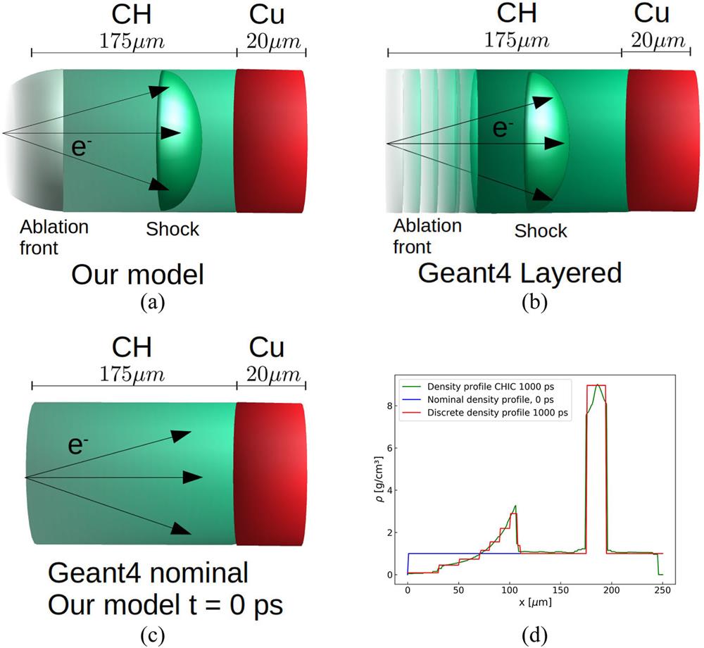
Fig. 1. Schematic representations of the target configuration used in the simulations performed. (a) Target used in simulations 1 and 2 performed with our MC model. The target configuration is extracted from CHIC simulations at four different times (250, 500, 750, and 1000 ps), and electrons are launched at the critical density. (b) Layered target used in simulation 3 performed with Geant4. The target is composed of several layers with increasing density, to reproduce the ablated and shocked regions. The density profile along the cylinder axis reproduces discretely the profile extracted from CHIC, as shown by the red curve in (d), for the case at 1000 ps. (c) Target used in the nominal Geant4 simulation and in the simulation with our MC code at 0 ps. This target is composed of a CH ablator of thickness 175 µm and density 1 g/cm³, followed by a copper plate of thickness 20 µm, as in the OMEGA experiment presented in Ref. 16. The density profile along the cylinder axis of this target is shown by the blue curve in (d). (d) Density profiles along the cylinder axis used in simulations 1 and 2 at 1000 ps (green curve), in simulation 3 (red curve), and in the nominal Geant4 simulation and in the simulation at 0 ps with our model (blue curve).

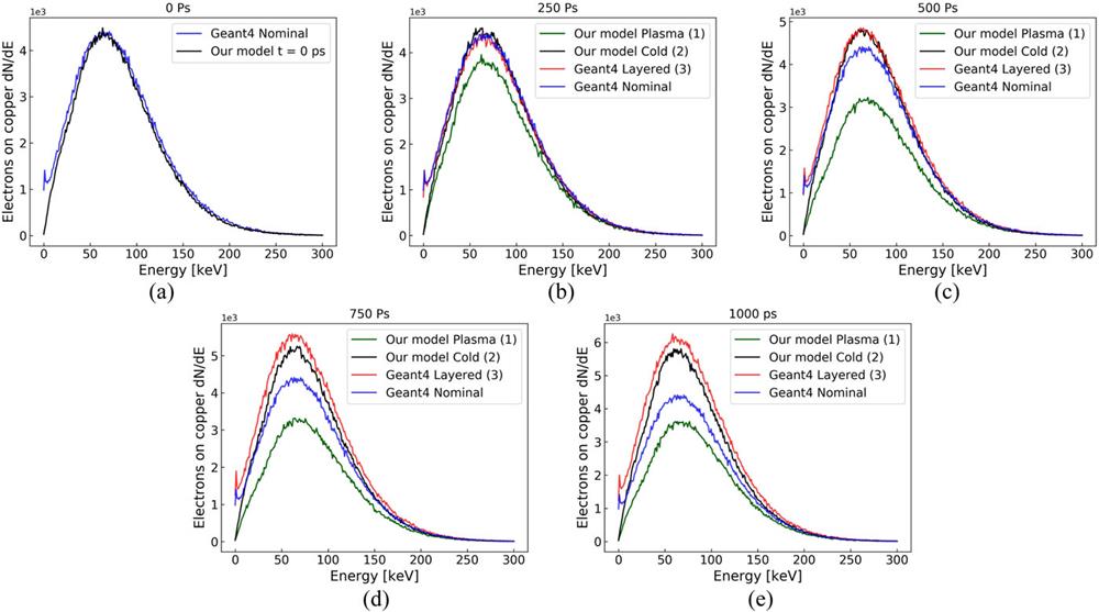
Fig. 2. Spectra of energetic electrons impinging on the copper plate as predicted by the simulations at five different times: (a) 0 ps (cold unablated target); (b) 250 ps; (c) 500 ps; (d) 750 ps; (e) 1000 ps. Electrons described energetically by a 2D Maxwellian function with T_h = 26 keV were launched at the critical density with an initial divergence of ±22°. The green curves are the spectra predicted by the plasma simulations (simulation 1). The black curves are the spectra predicted by our MC model in which the plasma effects have been turned off and electrons propagate according to the cold model (simulation 2). The blue curves are the spectra predicted by Geant4 for the nominal target configuration (175 µm, 1 g/cm³ CH–20 µm Cu). The red curves are the spectra predicted by Geant4 for a layered target that reproduces the density profile extracted from CHIC (simulation 3).

Fig. 3. Stopping power in polystyrene (1.05 g/cm³) as a function of electron kinetic energy in the plasma case with T = 10 eV (red curve) and the cold case (black curve). The plasma stopping power was computed according to the formulas presented in Paper I,¹⁷ while the cold stopping power was taken from the NIST database.³⁷

Fig. 4. Electron spectra impinging on the copper plate predicted by a plasma simulation in which the nuclear potential is screened by the residual electronic structure and other plasma particles (simulation 1, green curve) and a plasma simulation in which the nuclear potential is screened only by the electronic structure (brown curve). The simulations used the target profile extracted from CHIC at 500 ps. As input, electrons were described by a 2D Maxwellian function with T_h = 26 keV, launched at the critical density with an initial divergence of ±22°.

Fig. 5. Energetic electron spectra impinging on the copper plate predicted by a plasma simulation (simulation 1, green curve) and by a simulation in which the diffusion on plasma electrons is neglected (brown curve). The simulations used the target profile extracted from CHIC at 500 ps. As input, electrons were described by a 2D Maxwellian function with T_h = 26 keV, launched at the critical density with an initial divergence of ±22°.

Fig. 6. Electron spectra impinging on the copper plate with both hard and soft collisions considered (green curve), with hard collisions neglected (brown curve), and with beam diffusion neglected, i.e., with electrons propagating along straight lines (violet curve). The input spectrum was a Maxwellian function with T_h = 26 keV and an initial divergence of ±22°. The target hydrodynamic profile was extracted from a CHIC simulation at 500 ps.

Fig. 7. Electron spectra impinging on the copper plate with both primary and secondary particles (blue curve) and with only secondary electrons considered (black curve) according to Geant4 simulations. The input spectrum was a Maxwellian function with T_h = 26 keV and an initial divergence of ±22°. The simulations were conducted assuming the nominal target configuration (175 µm, 1 g/cm³ CH–20 µm Cu).

Fig. 8. Parameters T_h and N_e that reproduce the K_α signal on the ZnVH spectrometer in the experiment from Ref. 16 according to Geant4 simulations. The blue curve is from the nominal Geant4 simulation (i.e., a cold target composed of 175 µm CH and 20 µm Cu), and the red curve is for the plasma case. The Geant4 library used to compute the K_α was Livermore. The predicted hot-electron temperatures are ∼5% greater for the plasma case than for the cold case, while the difference in the parameter N_e does not exceed 30%. These percentages are indicated by the error bars.

Fig. 9. (a) Laser pulse used to implode the capsule. The pulse consists of a low-intensity compression beam followed by a high-intensity spike launched at 13.6 ns. The spike has duration of 1 ns. The total energy contained in the beam is around ∼350 kJ. (b) Schematic of the setup for the MC simulation and the geometric characteristics of the hot-electron beam.

Fig. 10. Adiabat as a function of shell radius, computed from the CHIC simulation at 13.6 ns. The positions of the shock front, the inner part of the shell, and the hotspot are indicated by the black, red, and green curves, respectively.

Fig. 11. Volumetric energy deposition along the capsule radius (blue curves) and density profile of the imploding capsule as a function of capsule radius (red curves). The capsule center is at r = 0 µm, and the shock is moving from right to left. (a) and (b) Simulations performed with f_e1 (see Table I) and target hydrodynamic profiles extracted from CHIC at 13.6 and 14.35 ns, respectively. (c) and (d) Simulations performed with f_e2 and target hydrodynamic profiles extracted from CHIC at 13.6 and 14.35 ns, respectively. Data are taken from simulations in which the hot-electron beam was initialized with a divergence of ±22° and a spot of diameter 1580 µm. The absolute values of energy deposited shown on the left vertical axis are not rescaled to take account of the real laser energy and they are not meaningful.

Fig. 12. Inner shell adiabat α_inn as a function of the hot-electron temperature T_h and the laser to hot-electron energy conversion efficiency η. The values of α_inn were calculated at the end of the implosion according to Eq. (4). Geometrically, the hot electrons were initialized with a beam divergence of ±22° and a spot of diamater 1580 µm. The red line delimits the region in which α_inn ≤ 1.8, while the green line delimits the region in which α_inn < 2.3. The red and light blue triangles indicate the hot-electron characteristics obtained experimentally at OMEGA-EP¹⁶ and LMJ,^15,44,45 respectively.

Table 1. Hot-electron temperatures T_h and laser to hot-electron conversion efficiencies η used as input in the simulations. The values of T_h are based on the experimental findings in Ref. 16 or used in Ref. 19. The values of α_inn at shock convergence, computed according to our MC simulations, are reported for the different beam geometries considered: an initial spot of diameter S = 1580 µm with divergence Div = 0°, ±22°, or ±45°, and an initial spot of S = 720 µm with Div = 0°. The last row shows the value of α_inn at shock convergence reported in Ref. 19. The value of the adiabat at the shock launch time was 1.7.