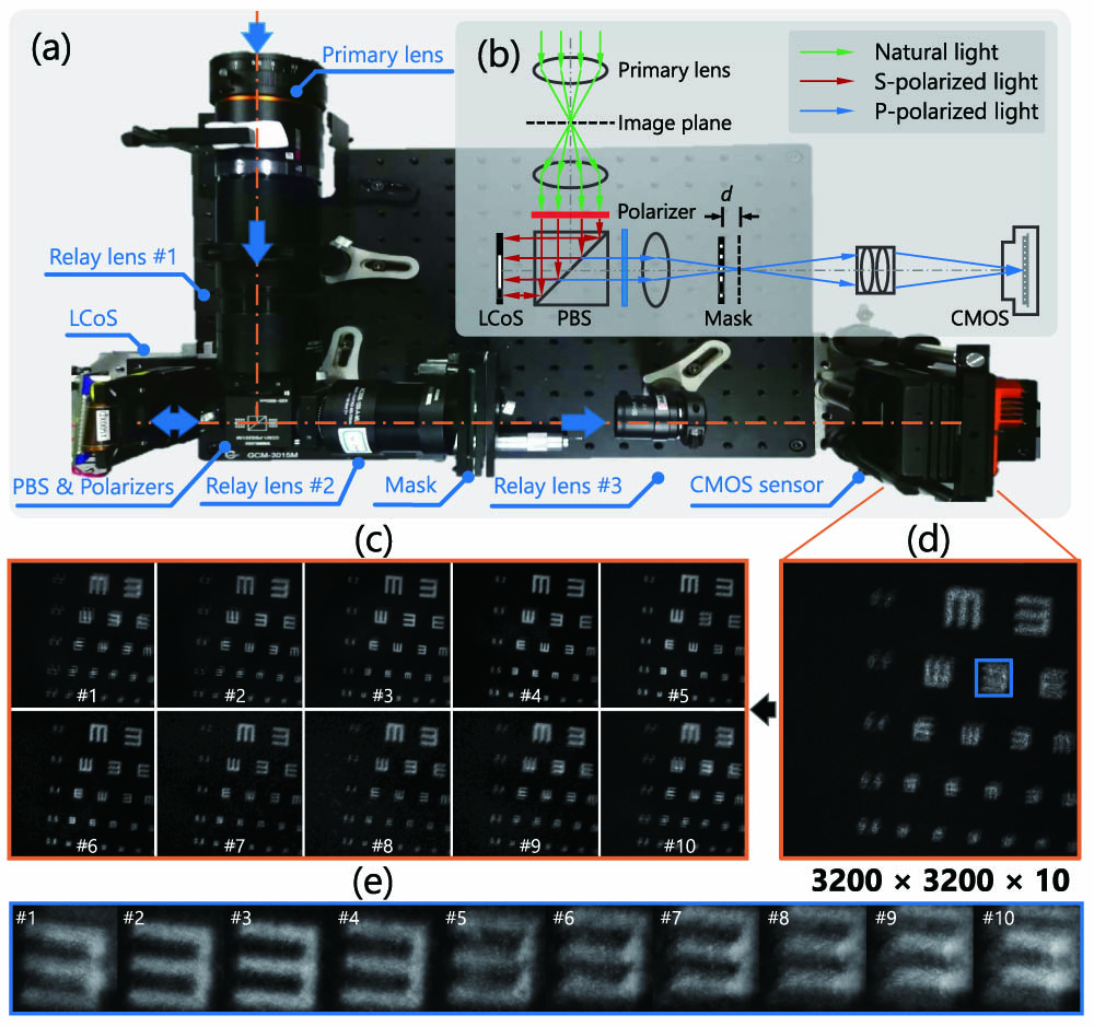
Fig. 1. Our 10-mega-pixel video SCI system (a) and the schematic (b). Ten high-speed (200 fps) high-resolution (3200×3200 pixels) video frames (c) reconstructed from a snapshot measurement (d), with motion detail in (e) for the small region in the blue box of (d). Different from existing solutions that only use an LCoS or a mask (thus with limited spatial resolution), our 10-mega-pixel spatio-temporal coding is generated jointly by an LCoS at the aperture plane and a static mask close to the image plane.

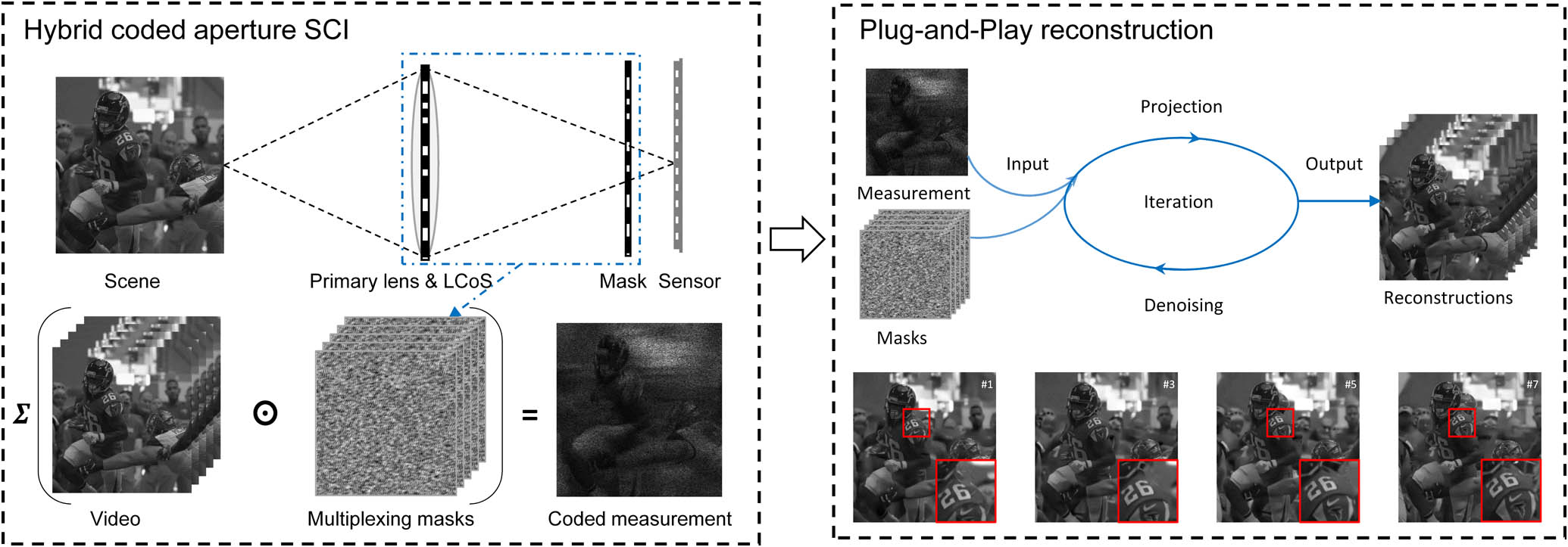
Fig. 2. Pipeline of the proposed large-scale HCA-SCI system (left) and the PnP reconstruction algorithms (right). Left: During the encoded photography stage, a dynamic low-resolution mask at the aperture plane and a static high-resolution mask close to the sensor plane work together to generate a sequence of high-resolution codes to encode the large-scale video into a snapshot. Right: In the decoding, the video is reconstructed under a PnP framework incorporating deep denoising prior and TV prior into a convex optimization (GAP), which leverages the good convergence of GAP and the high efficiency of the deep network.

Fig. 3. Illustration of the multiplexed mask generation. For the same scene point, its images generated by different sub-apertures (marked as blue, yellow, and red, respectively) intersect the mask plane with different regions and are thus encoded with corresponding (shifted) random masks before summation at the sensor. The multiplexing would raise the light flux for high SNR recording, while doing so only with slight performance degeneration.

Fig. 4. Multiplexing pattern schemes used in our experiments (taking Cr=6 for an example). Top row: multiplexing patterns for simulation experiments. Each pattern contains 50% open sub-apertures, and each sub-aperture is a 512×512 binning macro pixel on the LCoS. Bottom row: multiplexing patterns for real experiments. Each pattern contains an open circle with a radius of about 400 pixels, and the circles in adjacent patterns have a rotation of 360/Cr degrees.

Fig. 5. Reconstruction results and comparison with state-of-the-art algorithms on simulated data at different resolutions (left: 256×256, middle: 512×512, right: 1024×1024) and with different compression ratios (top: Cr=10, bottom: Cr=20). The BIRNAT results are not available for 512×512 and 1024×1024 since the model training will be out of memory. See Visualization 1, Visualization 2, Visualization 3, Visualization 4, Visualization 5, and Visualization 6 for the reconstructed videos.

Fig. 6. Noise robustness comparison between multiplexed and non-multiplexed masks.

Fig. 7. Reconstruction results of the PnP–TV–FastDVDNet on real data captured by our HCA-SCI system (Cr=6, 10, 20, and 30). Note the full frames are of 3200×3200, and we plot small regions about 400×400 in size to demonstrate the high-speed motion.

Fig. 8. Reconstruction comparison between the GAP–TV, PnP–FFDNet, and PnP–TV–FastDVDNet on real data captured by our HCA-SCI system (Cr=6, 10, 20, and 30). Note the full frames are of 3200×3200, and we plot small regions 512×512 in size to demonstrate the high-speed motion. See Visualization 7 for the reconstructed videos.

Table 1. Average Results of PSNR in dB (left entry in each cell) and SSIM (right entry in each cell) by Different Algorithms (Cr=10)^a

Table 2. Average Results of PSNR in dB (left entry in each cell) and SSIM (right entry in each cell) by Different Algorithms (Cr=20)^a

Table 3. PnP–TV–FastDVDNet for HCA-SCI