
Zhihong Zhang, Chao Deng, Yang Liu, Xin Yuan, Jinli Suo, Qionghai Dai, "Ten-mega-pixel snapshot compressive imaging with a hybrid coded aperture," Photonics Res. 9, 2277 (2021)
- Photonics Research
- Vol. 9, Issue 11, 2277 (2021)
Abstract
1. INTRODUCTION
Recent advances in machine vision with applications in robotics, drones, autonomous vehicles, and cellphones have brought high-resolution images into our daily lives. However, high-speed high-resolution videos are facing the challenge of low throughput due to the limited frame rate of existing cameras working at the high-resolution mode, although they have wide applications in various fields such as physical phenomena observation, biological fluorescence imaging, and live broadcast of sports. This is further limited by the memory, bandwidth, and power. Thus, we aim to address this challenge here by building a high-speed, high-resolution imaging system using compressive sensing. Specifically, our system captures the high-speed scene in an encoded way, thus maintaining the low bandwidth during capture. Next, reconstruction algorithms are employed to reconstruct the high-speed, high-resolution scenes to achieve high throughput. Note that although the idea of video compressive sensing has been proposed before, scaling it up to 10 mega pixels in spatial resolution presents the challenges of both hardware implementation and algorithm development. Figure 1 shows a real high-speed scene captured by our newly built camera.
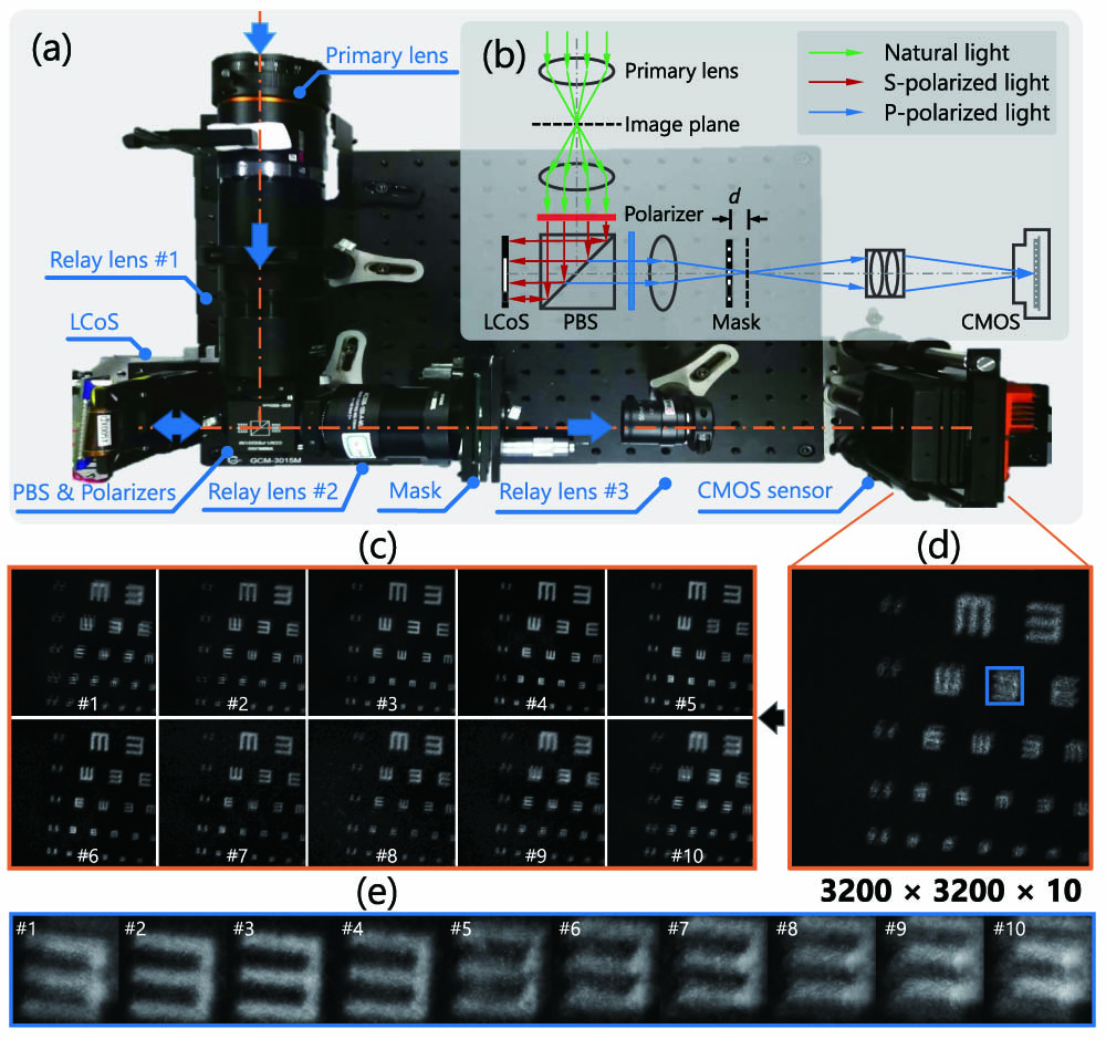
Figure 1.Our 10-mega-pixel video SCI system (a) and the schematic (b). Ten high-speed (200 fps) high-resolution (
While 10-mega-pixel lenses and sensors are both available, the main challenge for high-speed and high-resolution imaging lies in the deficient processing capability of current imaging systems. Massive data collected from high-speed high-resolution recording imposes dramatic pressure on the system’s storage and transmission modules, thus making it impossible for long-time capturing. In recent decades, the boosting of computational photography provides researchers with creative ideas and makes breakthroughs in many imaging-related fields such as super-resolution [1–3], deblurring [4–6], and depth estimation [7–9]. Regarding the high throughput imaging, snapshot compressive imaging (SCI) has been proposed and become a widely used framework [10–12]. It aims to realize the reconstruction of high-dimensional data such as videos and hyper-spectral images from a single-coded snapshot captured by a two-dimensional (2D) detector. A video SCI system is typically composed of an objective lens, a temporally varying mask, a monochrome or color sensor, and some extra relay lenses. During every single exposure, tens of temporal frames are modulated by corresponding temporal-variant masks and then integrated into a single snapshot. The high-dimensional data reconstruction in an SCI system can be formulated as an ill-posed linear model. Although different video SCI systems have been built [10,13–16], they are usually of low spatial resolution. By contrast, in this paper, we aimed to build a high-resolution video SCI system up to 10 mega pixels.
As mentioned above, the 10-mega-pixel lenses (including imaging lens and relay lens) and sensors are both commercialized products. Off-the-shelf reconstruction algorithms such as the recently developed plug-and-play (PnP) framework [17,18] can also meet our demands in most real applications. However, the 10-mega-pixel temporally varying mask is still an open challenge. Classical SCI systems usually rely on shifting masks produced by the lithography technique or dynamic patterns projected by the spatial light modulator (SLM), such as the digital micromirror device (DMD) or liquid crystal on silicon (LCoS), as temporally varying masks. The shifting mask scheme can provide high spatial resolution modulation, but it relies on the mechanical movement of the translation stage, which is inaccurate or unstable and can be hardly compact. For the masks generated by SLM or DMD, they can switch quickly with micro-mechanical controllers, but their resolution is generally limited to a mega-pixel level, which is difficult to scale up. To the best of our knowledge, there are few SCI systems that can realize
Sign up for Photonics Research TOC. Get the latest issue of Photonics Research delivered right to you!Sign up now
![]()
Figure 2.Pipeline of the proposed large-scale HCA-SCI system (left) and the PnP reconstruction algorithms (right). Left: During the encoded photography stage, a dynamic low-resolution mask at the aperture plane and a static high-resolution mask close to the sensor plane work together to generate a sequence of high-resolution codes to encode the large-scale video into a snapshot. Right: In the decoding, the video is reconstructed under a PnP framework incorporating deep denoising prior and TV prior into a convex optimization (GAP), which leverages the good convergence of GAP and the high efficiency of the deep network.
2. RELATED WORK
SCI has been proposed to capture high-dimensional data such as videos and hyper-spectral images from a single low-dimensional coded measurement. The underlying principle is to modulate the scene at a higher frequency than the camera frame rate, and then, the modulated frames are compressively sampled by a low-speed camera. Following this, inverse algorithms are employed to reconstruct the desired high-dimensional data [12].
Various video SCI systems have been developed recently [10,13–15,22–24], and the differences among these implementations mainly lie in the coding strategies. Typically, video SCI systems contain the same components as traditional imaging systems, except for several extra relay lenses and a modulation device that generates temporal-variant masks to encode the image plane. An intuitive approach is to directly use a DMD [15,22] or an LCoS [13,14], which can project given patterns with an assigned time sequence, on the image plane for image encoding. A substitute approach in early work is to simply replace the modulation device with a physically shifting lithography mask driven by a piezo [10]. There are also some indirect modulation methods proposed in recent work [23,24], which takes advantage of the temporal shifting feature of rolling shutter cameras or streak cameras for the temporal-variant mask generation.
Parallel to these systems, different algorithms are proposed to improve the SCI reconstruction performance. Since the inverse problem is ill-posed, different prior constrains such as TV [25], sparsity [10,13,14,16], self-similarity [26], and Gaussian mixture model [27,28] are employed, forming widely used TwIST [29], GAP–TV [25], DeSCI [26], and some other reconstruction algorithms. Generally, algorithms based on iterative optimization have high computational complexity. Inspired by advances of deep learning, some learning-based reconstruction approaches are proposed and boost the reconstruction performance to a large extent [15,30–34]. Recently, a sophisticated reconstruction algorithm BIRNAT [30] based on recurrent neural network has led to state-of-the-art reconstruction performance with a significant reduction on the required time compared with DeSCI. However, despite the highest reconstruction quality achieved by learning-based methods, their main limitation is in the inflexibility resulting from inevitable training process and requirement for large-scale training data when changing encoding masks or data capture environment. Other learning-based methods such as MetaSCI [31] try to utilize meta-learning or transfer learning to realize fast mask adaption for SCI reconstruction with different masks, but the time cost is still unacceptable on the 10-mega-pixel SCI data. To solve the trilemma of reconstruction quality, time consumption, and algorithm flexibility, a joint framework of iterative and learning-based methods called PnP [17] is proposed. By integrating pre-trained deep denoisers as the prior terms into certain iterative optimization process such as generalized alternating projection (GAP) [35] and alternating direction method of multiplier (ADMM) [36], PnP-based approaches combine the advantages of both frameworks and realize the trade-off between speed, quality, and flexibility.
In this paper, we build a novel video SCI system using a hybrid coded aperture, composed of an LCoS and a physical mask shown in Fig. 1. Moreover, we modify the PnP algorithm to fit our system, leading to better results than the method proposed in Ref. [17].
3. SYSTEM
A. Hardware Implementation
The hardware setup of our HCA-SCI system is depicted in Fig. 1. It consists of a primary lens (HIKROBOT, MVL-LF5040M-F,
It is worth noting that the active area of the LCoS and the position of the lithography mask should be carefully adjusted. The active area of the LCoS should be as large as possible meanwhile to ensure it to serve as the aperture stop of the whole system, so that it can provide a higher light efficiency. As for the lithography mask, some fine tuning is needed to ensure that the mask’s projection on the image plane can generate a shifting when different parts of the aperture are open, and meanwhile, the shifting masks can still keep sharp. In our implementation, after extensive experiments, the mask is placed in front of the second image plane with a distance of 80 μm, which is a good trade-off between the sharpness and the shift.
B. Encoding Mask Generation
The aperture of the system (i.e., the activated area of the LCoS) can be divided into several sub-apertures according to the resolution of the LCoS after pixel binning, and each sub-aperture corresponds to a light beam propagating toward certain directions. As shown in Fig. 3, because the lithography mask is placed in front of the image plane, when different sub-apertures are turned on, the light beams from the corresponding sub-apertures will project the mask onto different parts of the image plane, which can thus generate corresponding shifting encoding masks. In practice, to enhance the light throughput, multiple sub-apertures will be turned on simultaneously in one frame by assigning the LCoS with a specific multiplexing pattern to obtain a single multiplexing encoding mask. In addition, in different frames, different combinations of the sub-apertures are applied to generate different multiplexing encoding masks. Generally, we turn on 50% of the sub-apertures in one multiplexing pattern. In this multiplexing case, the final encoding mask on the image plane will be the summation of those shifting masks provided by the corresponding sub-apertures.
![]()
Figure 3.Illustration of the multiplexed mask generation. For the same scene point, its images generated by different sub-apertures (marked as blue, yellow, and red, respectively) intersect the mask plane with different regions and are thus encoded with corresponding (shifted) random masks before summation at the sensor. The multiplexing would raise the light flux for high SNR recording, while doing so only with slight performance degeneration.
C. Mathematical Model
Mathematically, the encoding mask generation process can be modeled as a multiplexing of shifting masks. Let
D. System Calibration
Although pixel-wise modulation is involved in SCI systems, there is no need for pixel-to-pixel alignment during system building, as we can get the precise encoding patterns through an end-to-end calibration process prior to data capture. To be specific, we place a Lambertian white board at the objective plane, and provisionally take away the lithography mask. Then, an illumination pattern
4. RECONSTRUCTION ALGORITHM
The reconstruction of high-speed videos from the snapshot-coded measurement is an ill-posed problem. As mentioned before, to solve it, different priors and frameworks have been employed. Roughly, the algorithms can be categorized into the following three classes [12]: i) regularization (or priors)-based optimization algorithms with well-known methods such as TwIST [29], GAP–TV [25], and DeSCI [26]; ii) end-to-end deep-learning-based algorithms [15,32,34], such as BIRNAT [30], which reaches state-of-the-art performance, and recently developed MetaSCI [31] that uses meta-learning to improve adaption capability for different masks in SCI reconstruction; and iii) PnP algorithms that use deep-denoising networks in the optimization framework such as ADMM and GAP.
Among these, regularization-based algorithms are usually too slow, and end-to-end deep learning networks need a large amount of data and also a long time to train the network, in addition to showing inflexibility (i.e., re-training being required for a new system). Although recent works such as MetaSCI [31] try to mitigate this problem with meta-learning or transfer learning and thus march forward to a large-scale SCI problem with a patch-wise reconstruction strategy, it still takes a long time for the training and adaption of 10-mega-pixel-scale SCI reconstruction. For example, MetaSCI takes about 2 weeks for the
In the following, we review the main steps of PnP–GAP [17] and then present our PnP–TV–FastDVDNet algorithm for HCA-SCI in Algorithm 1.
A. PnP–GAP
In GAP, the SCI inversion problem is modeled as
B. PnP–TV–FastDVDNet
Recall that solving
| 1: Initialize: |
| 2: |
| 3: Update |
| 4: Update |
| 5: |
| 6: |
| 7: |
| 8: |
| 9: |
Table 3. PnP–TV–FastDVDNet for HCA-SCI
In this paper, considering the high video denoising performance of recently proposed FastDVDNet [21], we jointly employ the TV denoiser and the FastDVDNet denoiser in a PnP–GAP framework, implementing a reconstruction algorithm of PnP–TV–FastDVDNet, which involves cascading and series denoising processes. The algorithm pipeline is shown in Algorithm 1. In each iteration, the updating of
5. RESULTS
In this section, we conduct a series of experiments on both simulation and real data to validate the feasibility and performance of our proposed HCA-SCI system. Four reconstruction algorithms, including iterative-optimization-based algorithm GAP–TV [25], plug-and-play-based algorithm PnP–FFDNet [17], our proposed PnP–TV–FastDVDNet, and the state-of-the-art learning-based algorithm BIRNAT [30] are employed.
A. Multiplexing Pattern Design
Multiplexing pattern design plays an important role in our HCA-SCI system. In simulation, we used the random squares multiplexing scheme (shown in the first row of Fig. 4), which contains 12 sub-apertures with each sub-aperture containing
![]()
Figure 4.Multiplexing pattern schemes used in our experiments (taking
Currently, the design of the multiplexing patterns is heuristic, and the challenge of the algorithm-based multiplexing pattern design mainly lies in the large size of the multiplexing pattern (
B. Reconstruction Comparison between Different Algorithms on Simulation Datasets
To investigate the reconstruction performance of different algorithms on the proposed HCA-SCI system, we first perform experiments on simulated datasets, which involve three different scales of
The reconstruction peak signal to noise ratio (PSNR) and structural similarity index measure (SSIM) for each algorithm are summarized in Tables 1 and 2 for
Average Results of PSNR in dB (left entry in each cell) and SSIM (right entry in each cell) by Different Algorithms (
| Scales | Algorithms | Football | Hummingbird | ReadySteadyGo | Jockey | YachtRide | Average |
|---|---|---|---|---|---|---|---|
| GAP–TV | 27.82, 0.8280 | 29.24, 0.7918 | 23.73, 0.7499 | 31.63, 0.8712 | 26.65, 0.8056 | 27.81, 0.8093 | |
| PnP–FFDNet | 27.06, 0.8264 | 25.52, 0.6912 | 21.68, 0.6859 | 31.14, 0.8493 | 23.69, 0.7035 | 25.82, 0.7513 | |
| BIRNAT | 34.67, 0.9719 | 34.33, 0.9546 | 29.50, 0.9389 | 36.24, 0.9711 | 31.02, 0.9431 | 33.15, 0.9559 | |
| GAP–TV | 29.19, 0.8854 | 28.32, 0.7887 | 25.94, 0.7918 | 31.30, 0.8718 | 26.59, 0.7939 | 28.27, 0.8263 | |
| PnP–FFDNet | 28.57, 0.8952 | 28.02, 0.8363 | 24.32, 0.7457 | 29.81, 0.8248 | 23.45, 0.6793 | 26.83, 0.7963 | |
| GAP–TV | 30.63, 0.9022 | 29.16, 0.8459 | 28.92, 0.8698 | 31.59, 0.8953 | 29.03, 0.8470 | 29.87, 0.8720 | |
| PnP–FFDNet | 29.87, 0.9023 | 27.70, 0.7869 | 27.70, 0.8483 | 29.88, 0.8412 | 25.55, 0.7211 | 28.14, 0.8200 | |
BIRNAT fails at large-scale due to limited GPU memory.
Average Results of PSNR in dB (left entry in each cell) and SSIM (right entry in each cell) by Different Algorithms (
| Scales | Algorithms | Football | Hummingbird | ReadySteadyGo | Jockey | YachtRide | Average |
|---|---|---|---|---|---|---|---|
| GAP–TV | 25.01, 0.7544 | 26.33, 0.6893 | 20.48, 0.6326 | 28.13, 0.8318 | 23.56, 0.7129 | 24.70, 0.7242 | |
| PnP–FFDNet | 21.67, 0.6657 | 22.13, 0.5835 | 17.27, 0.5340 | 27.78, 0.7994 | 20.39, 0.6024 | 21.85, 0.6370 | |
| BIRNAT | 27.91, 0.9021 | 28.58, 0.8800 | 23.79, 0.8279 | 31.35, 0.9467 | 26.14, 0.8585 | 27.55, 0.8830 | |
| GAP–TV | 23.97, 0.8179 | 24.50, 0.6719 | 22.12, 0.6975 | 26.99, 0.8297 | 23.13, 0.6930 | 24.14, 0.7420 | |
| PnP–FFDNet | 22.00, 0.7661 | 23.62, 0.7245 | 19.35, 0.6133 | 25.32, 0.7924 | 19.48, 0.5418 | 21.95, 0.6876 | |
| GAP–TV | 24.82, 0.8353 | 25.53, 0.7296 | 24.98, 0.8128 | 26.63, 0.8388 | 25.80, 0.7759 | 25.55, 0.7985 | |
| PnP–FFDNet | 23.55, 0.8098 | 23.02 0.6039 | 22.48, 0.7702 | 24.48, 0.7968 | 21.67, 0.6414 | 23.04, 0.7244 | |
BIRNAT fails at large-scale due to limited GPU memory.
![]()
Figure 5.Reconstruction results and comparison with state-of-the-art algorithms on simulated data at different resolutions (left:
C. Validation of Multiplexed Shifting Mask’s Noise Robustness on Simulation Datasets
As mentioned in Section 5.B, our proposed HCA-SCI system leverages multiplexing strategy for the improvement of light throughput, which can thus gain a higher signal-to-noise ratio (SNR) and enhance the system’s robustness to noise in real-world applications. In this subsection, we conduct a series of experiments on simulation datasets containing different levels of noise to compare the reconstruction performance of multiplexed shifting masks used in HCA-SCI and non-multiplexed ones. The
The change of reconstruction PSNR over increasing noise levels is shown in Fig. 6. As can be seen from the figure, shifting masks with no multiplexing outperform the multiplexed ones when there is no noise, which is probably because the multiplexing operation brings in some correlation among the masks that is not desired for the encoding and reconstruction. However, as the noise increases, the superiority in SNR of the multiplexing scheme shows up, and the reconstruction PSNR of non-multiplexed shifting masks drops rapidly, while that of the multiplexed masks decreases more slowly and exceeds the PSNR of the non-multiplexed ones. In real scenes, noise is inevitable, and as it increases, it will also have a significant impact on the reconstruction process until totally disrupting the reconstruction. Thus, the multiplexing strategy leveraged in HCA-SCI can equip the physical system with more robustness in real applications, especially those at relatively large noise levels.
![]()
Figure 6.Noise robustness comparison between multiplexed and non-multiplexed masks.
D. Real-Data Results
We built a 10-mega-pixel snapshot compressive camera prototype illustrated in Fig. 1 for dynamic video recording. Empirically, the multiplexing patterns (shown in the second row of Fig. 4) projected by the LCoS are designed to be rotationally symmetric, which ensures the consistency in the final coding patterns and provides an adequate incoherence among these masks. Before acquisition, we first calibrate the groups of coding masks with a Lambertian whiteboard placed at the objective plane, and each calibrated pattern is averaged over 50 repetitive snapshots to suppress the sensor noise. Then, during data capture, the camera operates at a fixed frame rate of 20 fps when
Three moving test charts printed on A4 papers are chosen as the dynamic objects. In Fig. 7, we show the coded measurements and final reconstruction of the test charts. From that, one can see that the proposed HCA-SCI system and PnP–GAP–FastDVDNet reconstruction algorithm can effectively capture and restore the moving details of dynamic objects, which will be blurry when captured directly with conventional cameras. For the reconstruction of real data, we also find that, in some cases, the start and end frames tend to be blurry (refer to real-data results of
![]()
Figure 7.Reconstruction results of the PnP–TV–FastDVDNet on real data captured by our HCA-SCI system (
We further compare the reconstruction of GAP–TV, PnP–FFDNet, and PnP–TV–FastDVDNet on real datasets captured by our HCA-SCI system. From the reconstruction results shown in Fig. 8, we can find that when
![]()
Figure 8.Reconstruction comparison between the GAP–TV, PnP–FFDNet, and PnP–TV–FastDVDNet on real data captured by our HCA-SCI system (
6. CONCLUSION
We have proposed a new computational imaging scheme capable of capturing 10-mega-pixel videos with low bandwidth and developed corresponding algorithms for computational reconstruction, providing a high-throughput (up to 4.6 × 10⁹ voxels per second) solution for high-speed, high-resolution videos.
The hardware design bypasses the pixel count limitation of available spatial light modulators via joint coding at aperture and close to image plane. The results demonstrate the feasibility of high-throughput imaging under a snapshot compressive sensing scheme and hold great potential for future applications in industrial visual inspection or multi-scale surveillance.
So far, the final reconstruction is limited to 450 Hz since the hybrid coding scheme further decreases the light throughput to some extent, compared with conventional coding strategies. In the future, a worthwhile extension would be to introduce new photon-efficient aperture-coding devices to raise the SNR for coded measurements. Another limitation of the current system lies in the non-uniformity of the encoding masks along the radial direction, which is a common problem for large-scale imaging systems due to non-negligible off-axis aberration. Considering the challenge for improving optical performance of existing physical components, designing novel algorithms capable of SCI reconstruction with non-uniform masks may be economical and feasible. Meanwhile, time-efficient reconstruction algorithms and feasible multiplexing pattern design methods for large-scale (like 10-mega-pixel or even giga-pixel) SCI reconstruction are still an open challenge in the foreseeable future. Moreover, extending proposed imaging scheme for higher throughput (e.g., giga pixel) or other dimensions (e.g., light field, hyperspectral imaging) may also be a promising direction.
References
[1] G. Carles, J. Downing, A. R. Harvey. Super-resolution imaging using a camera array. Opt. Lett., 39, 1889-1892(2014).
[2] S. Farsiu, M. D. Robinson, M. Elad, P. Milanfar. Fast and robust multiframe super resolution. IEEE Trans. Image Process., 13, 1327-1344(2004).
[3] R. F. Marcia, R. M. Willett. Compressive coded aperture superresolution image reconstruction. IEEE International Conference on Acoustics, Speech and Signal Processing (ICASSP), 833-836(2008).
[4] T. S. Cho, A. Levin, F. Durand, W. T. Freeman. Motion blur removal with orthogonal parabolic exposures. IEEE International Conference on Computational Photography (ICCP), 1-8(2010).
[5] R. Raskar, A. Agrawal, J. Tumblin. Coded exposure photography: motion deblurring using fluttered shutter. ACM Trans. Graph., 25, 795-804(2006).
[6] C. Zhou, S. Nayar. What are good apertures for defocus deblurring?. IEEE International Conference on Computational Photography (ICCP), 1-8(2009).
[7] C. Zhou, S. Lin, S. K. Nayar. Coded aperture pairs for depth from defocus and defocus deblurring. Int. J. Comput. Vis., 93, 53-72(2011).
[8] A. Sellent, P. Favaro. Optimized aperture shapes for depth estimation. Pattern Recognit. Lett., 40, 96-103(2014).
[9] S. Suwajanakorn, C. Hernandez, S. M. Seitz. Depth from focus with your mobile phone. IEEE Conference on Computer Vision and Pattern Recognition (CVPR), 3497-3506(2015).
[10] P. Llull, X. Liao, X. Yuan, J. Yang, D. Kittle, L. Carin, G. Sapiro, D. J. Brady. Coded aperture compressive temporal imaging. Opt. Express, 21, 10526-10545(2013).
[11] A. Wagadarikar, R. John, R. Willett, D. Brady. Single disperser design for coded aperture snapshot spectral imaging. Appl. Opt., 47, B44-B51(2008).
[12] X. Yuan, D. J. Brady, A. K. Katsaggelos. Snapshot compressive imaging: theory, algorithms, and applications. IEEE Signal Process Mag., 38, 65-88(2021).
[13] D. Reddy, A. Veeraraghavan, R. Chellappa. P2C2: programmable pixel compressive camera for high speed imaging. IEEE Conference on Computer Vision and Pattern Recognition (CVPR), 329-336(2011).
[14] Y. Hitomi, J. Gu, M. Gupta, T. Mitsunaga, S. K. Nayar. Video from a single coded exposure photograph using a learned over-complete dictionary. International Conference on Computer Vision (ICCV), 287-294(2011).
[15] M. Qiao, Z. Meng, J. Ma, X. Yuan. Deep learning for video compressive sensing. APL Photon., 5, 030801(2020).
[16] X. Yuan, P. Llull, X. Liao, J. Yang, D. J. Brady, G. Sapiro, L. Carin. Low-cost compressive sensing for color video and depth. IEEE Conference on Computer Vision and Pattern Recognition (CVPR), 3318-3325(2014).
[17] X. Yuan, Y. Liu, J. Suo, Q. Dai. Plug-and-play algorithms for large-scale snapshot compressive imaging. IEEE/CVF Conference on Computer Vision and Pattern Recognition (CVPR), 1444-1454(2020).
[18] X. Yuan, Y. Liu, J. Suo, F. Durand, Q. Dai. Plug-and-play algorithms for video snapshot compressive imaging(2021).
[19] Y. Sun, X. Yuan, S. Pang. Compressive high-speed stereo imaging. Opt. Express, 25, 18182-18190(2017).
[20] L. I. Rudin, S. Osher, E. Fatemi. Nonlinear total variation based noise removal algorithms. Physica D, 60, 259-268(1992).
[21] M. Tassano, J. Delon, T. Veit. FastDVDnet: towards real-time deep video denoising without flow estimation. IEEE/CVF Conference on Computer Vision and Pattern Recognition (CVPR), 1351-1360(2020).
[22] C. Deng, Y. Zhang, Y. Mao, J. Fan, J. Suo, Z. Zhang, Q. Dai. Sinusoidal sampling enhanced compressive camera for high speed imaging. IEEE Trans. Pattern Anal. Mach. Intell., 43, 1380-1393(2021).
[23] L. Gao, J. Liang, C. Li, L. V. Wang. Single-shot compressed ultrafast photography at one hundred billion frames per second. Nature, 516, 74-77(2014).
[24] N. Antipa, P. Oare, E. Bostan, R. Ng, L. Waller. Video from stills: lensless imaging with rolling shutter. IEEE International Conference on Computational Photography (ICCP), 1-8(2019).
[25] X. Yuan. Generalized alternating projection based total variation minimization for compressive sensing. IEEE International Conference on Image Processing (ICIP), 2539-2543(2016).
[26] Y. Liu, X. Yuan, J. Suo, D. Brady, Q. Dai. Rank minimization for snapshot compressive imaging. IEEE Trans. Pattern Anal. Mach. Intell., 41, 2990-3006(2019).
[27] J. Yang, X. Yuan, X. Liao, P. Llull, D. J. Brady, G. Sapiro, L. Carin. Video compressive sensing using Gaussian mixture models. IEEE Trans. Image Process., 23, 4863-4878(2014).
[28] J. Yang, X. Liao, X. Yuan, P. Llull, D. J. Brady, G. Sapiro, L. Carin. “Compressive sensing by learning a Gaussian mixture model from measurements. IEEE Trans. Image Process., 24, 106-119(2015).
[29] J. Bioucas-Dias, M. Figueiredo. A new TwIST: two-step iterative shrinkage/thresholding algorithms for image restoration. IEEE Trans. Image Process., 16, 2992-3004(2007).
[30] Z. Cheng, A. Vedaldi, H. Bischof, R. Lu, T. Brox, Z. Wang, J.-M. Frahm, H. Zhang, B. Chen, Z. Meng, X. Yuan. BIRNAT: bidirectional recurrent neural networks with adversarial training for video snapshot compressive imaging. European Conference on Computer Vision, 258-275(2020).
[31] Z. Wang, H. Zhang, Z. Cheng, B. Chen, X. Yuan. MetaSCI: scalable and adaptive reconstruction for video compressive sensing. IEEE/CVF Conference on Computer Vision and Pattern Recognition (CVPR), 2083-2092(2021).
[32] M. Iliadis, L. Spinoulas, A. K. Katsaggelos. Deep fully-connected networks for video compressive sensing. Digit. Signal Process., 72, 9-18(2018).
[33] K. Kulkarni, S. Lohit, P. Turaga, R. Kerviche, A. Ashok. ReconNet: non-iterative reconstruction of images from compressively sensed measurements. IEEE Conference on Computer Vision and Pattern Recognition (CVPR), 449-458(2016).
[34] J. Ma, X.-Y. Liu, Z. Shou, X. Yuan. Deep tensor ADMM-net for snapshot compressive imaging. IEEE/CVF International Conference on Computer Vision (ICCV), 10222-10231(2019).
[35] X. Liao, H. Li, L. Carin. Generalized alternating projection for weighted-
[36] S. Boyd, N. Parikh, E. Chu, B. Peleato, J. Eckstein. Distributed optimization and statistical learning via the alternating direction method of multipliers. Foundations Trends Mach. Learn., 3, 1-122(2011).
[37] S. Jalali, X. Yuan. Compressive imaging via one-shot measurements. IEEE International Symposium on Information Theory, 416-420(2018).
[38] S. Jalali, X. Yuan. Snapshot compressed sensing: performance bounds and algorithms. IEEE Trans. Inf. Theory, 65, 8005-8024(2019).
[39] K. Zhang, W. Zuo, L. Zhang. FFDNet: toward a fast and flexible solution for CNN based image denoising. IEEE Trans. Image Process., 27, 4608-4622(2018).
[40] S. Gu, L. Zhang, W. Zuo, X. Feng. Weighted nuclear norm minimization with application to image denoising. IEEE Conference on Computer Vision and Pattern Recognition (CVPR), 2862-2869(2014).
[41] A. Mercat, M. Viitanen, J. Vanne. UVG dataset: 50/120 fps 4K sequences for video codec analysis and development. 11th ACM Multimedia Systems Conference, 297-302(2020).


Set citation alerts for the article
Please enter your email address

© Copyright 2018-2021 | Chinese Laser Press. All Rights Reserved 沪ICP备15018463号-20