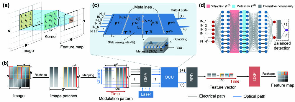
Fig. 1. Principle of optical image convolution based on OCU. (a) Operation principle of 2D convolution. A fixed kernel with size of H×H slides over the image with size of N×N by stride of S and does weighted addition with the image patches that are covered by the kernel, resulting in an extracted feature map with size of G×G, where G=⌊(N−H)/S+1⌋. (b) Optical image convolution architecture with OCU. An image is first flattened into patches according to the kernel size and sliding stride and then mapped into a modulation pattern confined with time and channel number, which modulates a coherent laser via a modulation array. The modulated light is sent to OCU to perform optical convolution, whose positive and negative results are subtracted by a balanced photodetector and reshaped by a DSP to form a new feature map. OMA, optical modulator array; BPD, balanced photodetector; DSP, digital signal processor. (c) Details of OCU. H2 waveguides are used to send a laser signal into a silicon slab waveguide with size of L1×L2, and layers of metaline are exploited successively with layer gap of L2, which are composed by well-arranged metaunits. Three identical silica slots with sizes of w1×w2×h are used to compose one metaunit with gap of g, and the period of metaunits is p. The phase modulation is implemented by varying w2. The transfer function of the diffraction in slab waveguide and phase modulation of metalines are denoted as F and T. (d) The feedforward neural network abstracted from the OCU model. Red and blue boxes denote diffractions and phase modulations of metalines; gray box represents intensitive nonlinear activation of complex-valued neural networks introduced by photodetection.

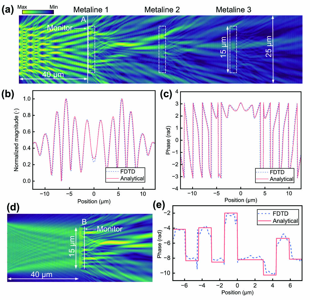
Fig. 2. (a) Optical field of the OCU evaluated by FDTD method. A monitor is set at Position A to receive the optical field of the incident light. (b) Magnitude and (c) phase response of the optical field at Position A (red solid curve) match well with the analytical model (purple dash curve) in Eq. (5). (d) Optical field of the metaline with incident light of a plane wave. A monitor is set behind the metaline at Position B to obtain its phase response. (e) The analytical model (purple dash curve) of Eq. (6) fits well with the FDTD calculation (red solid curve).

Fig. 3. Concept of structural reparameterization in deep learning. Network Structure 1 has a transfer function of F, which can be substituted equivalently by Network Structure 2, whose transfer function is G. Accordingly, both structures have the same outputs y under the same inputs of x.

Fig. 4. Training and the inference phase of an OCU to perform real-valued optical convolution with the idea of SRP in deep learning. (a) A 128×128 random pattern is utilized to generate a training pair for OCU model. The output feature vector of OCU model is supervised by the training label with the input of flattened image patches decomposed from the random pattern. (b) A 256×256 gray-scale image is reshaped to flattened patches and sent to the well-trained OCU to perform a real-valued convolution. OMA, modulator array; BPD, balanced photodetector; DSP, digital signal processor.

Fig. 5. Well-agreed convolution results between the ground truths and the outputs of OCUs with eight unique real-valued convolution kernels, with average PSNR of 36.58 dB. GT, ground truth.

Fig. 6. Architecture of oCNN for image classification. Images with size of N×N×C are first flattened into C groups of patches and concatenated as a data batch with size of G2×C·H2, according to the kernel size H, and then loaded to a modulator array with total C·H2 modulators in parallel. The modulated signal is split to q OCKs by an optical router, each of which contains C OCUs to generate C subfeature maps; then, all the subfeature maps of each OCK are summed up to form a final feature map. We refer to this process as an OCL, denoted by the blue dashed box. After OCL, the feature maps are further downsampled by a pooling layer, and multiple OCLs and pooling layers can be utilized to build deeper networks to manipulate more complicated tasks. A small-scale fully connected layer is used to give the final classification results. OMA, optical modulator array; OCK, optical convolution kernel; BPDA, balanced photodetector array; FM, feature map; FC, fully connected layer.

Fig. 7. Classification results of oCNNs for (a) fashion-MNIST and (b) CIFAR-4 data sets. Accuracies of 91.63% and 86.25% are obtained with oCNNs for the corresponding two data sets, which outperform their electrical counterparts with 1.14% and 1.75% respectively. (c) Classification performance evaluations on both data sets with respect to two main physical parameters of OCU: the number of metaunit per layer and the number of the exploited metaline layer. (d) 2D visualizations of the two applied data sets with t-distributed stochastic neighbor embedding (t-SNE) method.

Fig. 8. (a) Architecture of the proposed oDnCNN. A Gaussian noisy image with a known noise level is first flattened and modulated into a lightwave and then sent to oDnCNN, which is composed of three parts: input layer with OCL and ReLU; middle layer with an extra batch normalization between the two; and output layer with only an OCL. After the oDnCNN, a residual image is obtained, which is the extracted noise. By subtracting the noisy image with the extracted residual one, the clean image can be aquired. OCL, optical convolution layer; ReLU, rectified linear unit; BN, batch normalization. (b) The denoised result of Set12 data set leveraged by the proposed oDnCNN with noise level σ=20, giving much clearer textures and edges as the details show in red boxes. In this case, the average PSNR of the denoised images is 27.02 dB, compared with 22.10 dB of the noisy ones. NI, noisy images; DI, denoised images.

Fig. 9. Method of OCU’s scaling for computing multiple convolutions. (a) Computing with prototype OCU. N convolutions require N prototype OCUs, each of which represents one kernel. (b) Principle of scaling up the prototype. Optical diffraction in silicon slab waveguide provides spatially-varied field at the output facet of OCU, which enables the possibility for multiplexing multiple convolution operations spatially. (c) Computing with space-multiplexed OCU. N convolutions can be calculated by just one space-multiplexed OCU with its fitting target of a kernel matrix K=[K1,K2,…,KN], where Ki is a 1×H2 vector with i=1,2,…,N. SDM, space division multiplexing.

Fig. 10. Highly efficient optical deep learning framework with network rebranching and optical tensor core. Deep learning models are decomposed mathematically into two parts: trunk and branch, which carry the major and minor calculations of the model, respectively. The trunk part is computed by an optical tensor core with fixed weights, and the branch part is performed by a lightweight electrical network to reconfigure the model. OTC, optical tensor core; OTU, optical tensor unit.

Table 1. Performance Comparisons of the Proposed oDnCNN and E-net in Average PSNR, with Noise Level σ=10, 15, and 20

Table 2. Comparison of State-of-the-Art Integrated Photonic Computing Hardware^a