Earth’s surface is an intersectional study point of geology, hydrology, and meteorology. Geomorphologists have always been taking the most time to pay attention to the full use of Earth surface resources. Along with the development of the knowledge-based economy and sci-tech globalization, numerous approaches have been used to help understanding landform dynamics. Deeper insights into basic principles in turn suggest the interactions of various surface processes that represented by fluvial processes varying with climate processes need to be concentrated more due to the increase of extreme weather events attributed by human-induced global warming (Hansen et al., 2000). In general, rivers are thought of key links for connecting different landscape elements. Coordinating large number of river issues including the investigation of river dynamics and overall river management, is one of the most significant topics in many developing countries. However, extreme weather events impose a considerable burden upon balancing human activities and the sustainable utilization of earth’s resources (Wang et al., 2015). River is well known as a high complex system, we must face the fact that conquering nature is a phased process that requires a great deal of treatments for existing classical problems and some new difficulties on the local scale brought about by the inherent nonlinearity and abruptness in river system.

Some linear/nonlinear bend theories help us understand some unexplored nonlinear aspects of meandering channels for a long time. However, contradictions and limitations are inevitable in the development course of river theory. Driven by seasonal and abnormal events, the state of river channels is continuously changing with the development of hydrologic force, which undoubtedly makes us question the traditional model assumption that whether river could reach a dynamic equilibrium state subjecting to repeated sequence of external disturbances. The frequent occurrence of storms and floods adds to some confusions: how the morphology fluctuations and event characteristics relate to each other; whether it is reasonable to define a singular and dominant discharge to account for unsteady factors that affect the shape of landscape (Wolman and Ran, 1978), meanwhile as there also exists the objection that river structure may be an integrated result of historical disturbances (Graf, 1979), not a quasi-equilibrium state with flood disasters (Pittaluga and Seminara, 2011). Some researchers exploited the sensitivity of hydrological response of river channels to extreme rainfall events by natural experiment statistics or remote sensing in some specific areas (Bauch and Hickin, 2011; Harrison et al., 2017), but few mechanistic description to fluvial relationships for balancing engineering benefit and environmental protection in the planning and design of flood channels.

Recently, many physicists turned to system theory to study complicated dynamic process with biological and ecological factors to participate in. In particular, transfer function, a single-input single-output filter based on differential equations, has occupied a primary and central place within the fields of system analysis over time. Unlike some simple systems with specific components changing according to deterministic equations, river systems are observed to behave in a non-equilibrium manner with the characteristics of rich irregularity and interactivity. For this reason, scientists developed stochastic models, for example, the deformations of classic Transfer Function Noise models, for enhancing the forecast of river flows generated by rainfall (Liu, 2009; Wasimi and Mondal, 2005); some focused on describing the dynamic probability transformation of water quality constituents in river system (Boano et al., 2006); some investigated the random dynamics of riparian width and vegetation biomass with random discharge taken into account (Muneepeerakul et al., 2007; Tealdi et al., 2011); and there also exists the description of soil water balance dynamics over a schematic river basin based on a stochastic differential equation with the addition of rainfall forcing modeled by white noise instead of blind use of deterministic models (Manfreda and Fiorentino, 2008). In spite of its inherent shortcoming of unwieldy application, state space representations of multiple transfer function, namely, transfer matrix, still has been largely proposed as an alternative approach for the analysis of multiple-input multiple-output systems. River is a systemic, dynamic and multi-factor system. The above tools offer such an effective way for river basin management by incorporating the randomness of flow input into a probabilistic framework, which can be reasonably expected to help address extreme climate events.

Until now, the stochastic response of fluvial relationships is still lack of analysis as complete, accurate and reliable as possible. Different minimization theories and nonlinear dynamic analysis (Navratil and Albert, 2010; Yang et al., 1981; Xia et al., 2014) have been used to study the existing most famous hydraulic geometry relationship; while surprisingly, most applications only work on solving the parameters of the empirical equilibrium relations itself, the potential catastrophic of which triggered by events was few expected in a time of frequent occurrence of extreme weather. This relationship carries so vital information for a given river system that the present paper aims to open the new potentials of which based on stochastic differential equations. New insights will help future realization of effective and space saving measures so as to avoid lagging behind time schedules and to strengthen capacity for crisis response across catchments.

Classic theory presumed that the rivers are most powerfully shaped by water and sediment inflow at the bankfull stage where the river channel and floodplain become connected. Numerous geomorphologists focused on identifying the bankfull stage and defining a single dominant discharge as the bankfull discharge for river channels in equilibrium. Real-Riverworld experience, however, suggests that this problem was oversimplified and it is doubtful whether the rivers could evolve into a relative steady state. In the Lower Yellow River, Wu et al. (2008) investigated a sequence of transitional river states, and analyzed the phenomenon of delayed response of bankfull discharge to flow and sediment changes. Herein, the variation of bankfull discharge was described as an adjustment between the current value and its potential equilibrium value:

where Q_t is the bankfull discharge at time t; β is the rate at which the equilibrium state is being approached; ${{Q}_{e}}$is the equilibrium bankfull discharge represented by a formula that depends on flow discharge and suspended sediment concentration in flood season:

where Q_f, ${{\xi }_{f}}$, and C_tf are the mean discharge, incoming sediment coefficient, and suspended sediment concentration in flood season respectively; K, b, c are the unknown parameters.

Then for such channels, we can define a bankfull channel geometry group constituted by bankfull discharge, channel slope, width, depth and velocity in terms of simple power functions:

where S_t, B_t, D_t and U_t are the down-channel bed slope, cross-sectional channel width, depth and velocity in bankfull stage at time t respectively, and other coefficients and exponents are constants.

From the general view, Eqs.(3) can be simplified by:

where X_t is the typical bankfull channel geometry variable.

After taking the derivative of Eq.(4), we have:

Combining Eq.(5) and Eq.(1), then a deterministic differential equation set with respect to bankfull channel geometries are established:

However, highly organized river systems possess the characteristics of rich regularity and interactivity(Huggett, 2007), increasing non-equilibrium issues on account of continuing uncertainties from flow-sediment input and channel boundary conditions greatly reduce the effectiveness of deterministic models on reflecting the real river development. Considering real systems cannot completely eliminate external stochastic influence and then exist alone, stochastic differential equations (SDEs), which link probability theory and ordinary differential equation, could find applications in this kind of situation. Through randomizing models by adding one or more stochastic noise terms, SDEs improve the dynamical systems theory significantly and have had wide applicability in modeling various physical systems such as molecular dynamics, stock market fluctuations and even the dynamics of the astrophysical processes. Research on rivers also benefits from the development of the stochastic theory (Camporeale and Ridolfi, 2006; Manfreda and Fiorentino, 2008; Wasimi and Mondal, 2005), and have been given new intuitive interpretations. In view of such important generalization, we follow them to transform deterministic models (6) into stochastic models by introducing random noises on a given, fixed, time-interval [0, T]:

where Q^*_t and X^*_t are stochastic bankfull discharge and hydraulic geometry variable; $\overline{{{Q}_{t}}}$represents the average of stochastic discharge; $\zeta _{t}^{[1]}$and $\zeta _{t}^{[2]} $ are the same types of external random noise.

The classic SDEs usually use Gaussian white noise to describe the random noise terms. However, the main weakness of such processing is that Gaussian white noise only represents kind of continuous and stable stochastic excitation, it fails to describe the sudden changes of variables. In fact, white noise is equivalent to white light which consists of all different visible spectrums, multiple random noises are also involved in natural noise system. Not only is there Gaussian white noise existing, but also works in non-Gaussian ways. Non-Gaussian shot noise, or Poisson noise, is a typical type of impulse noise which carries some important sharp information and can be modeled by Poisson process. Many stochastic studies (Bruti-Liberati and Platen, 2006; Chalmers et al., 2008; Rong, 2006) found evidence of the importance of jumps and suggested to include Poisson jumps in SDEs. Moreover, consideration should also be given to nonlinearity. That is, at some point one variable may be likely to have unexpected overreactions on exponential level. Traditional linear thought model may be contradictory to the fact, that is, Real River systems are not machines, but living systems, just like molecular biology world, they may show some spontaneity and complexity. Studies (Leland et al., 1994) show that real system inputs can sometimes exhibit long-range dependence and self-similarity in these fields, and the fractional Brownian motion (fBm) is recommended as the typical stochastic process that possesses such characteristics (Decreusefond and Üstünel, 1999). Therefore, we may be able to try applying fractal theory into SDEs so as to better characterize the propagation of hydraulic geometries. Given the above, we use three types of combinations of popular noise models, including Gaussian white noise, Poisson noise, and Fractional white noise, to evaluate the effectiveness of SDEs-Eq.(7) in describing the dynamics of hydraulic geometries respectively. The details are as follow:

2.1.1 Single Gaussian white noise model

with discrete solution (Glasserman, 2004):

where σ₁, σ₂ are the diffusion parameters of the two stochastic models (Eqs. 8a and 8b), respectively; γ is exponent parameter; W represents uncorrelated multiplicative standard Gaussian white noise; Z represents independent standard normal random variable.

Here, we use a CKLS (Chan et al., 1992) type model to define the stochastic process of bankfull discharge, and a Black-Scholes (Black and Scholes, 1973) type model to describe the dynamic hydraulic geometry.

2.1.2 Compound Gaussian white noise plus Poisson noise model:

where V^j is the jump magnitude, N^j(λ^j) are independent Poisson processes with intensity parameters λ^j (j=u, d represent up- and down-jumps, respectively), the distribution of the logarithm of jump magnitudes (Y=ln(V)) is given by a mixed double exponential density function of form:

where ${{\eta }_{u}}>1$, ${{\eta }_{d}}>0$and \[0\le p=\frac{{{\lambda }^{u}}}{{{\lambda }^{u}}+{{\lambda }^{d}}},q=\frac{{{\lambda }^{d}}}{{{\lambda }^{u}}+{{\lambda }^{d}}}\le 1$.

Here, we use a combined approach to simulate the times (${{\tau }_{1}},{{\tau }_{2}},\ldots $) at which jumps occur, of which times difference ${{R}_{i+1}}={{\tau }_{i+1}}-{{\tau }_{i}}$can be generated from the exponential distribution with mean $1/\lambda $. $\lambda $ is estimated according to historical data (Tsai et al., 2014). Q^*_t and X^*_t evolve like an ordinary geometric Brownian motion from one jump moment to the next. Suppose a date t is included among the simulated dates, that is,${{\tau }_{i}}<t<{{\tau }_{i+1}}$, then the discrete solutions could be expressed as follows:

in which, $\begin{matrix} & \prod\limits_{j=u,d}{{{V}^{j}}(N_{1}^{j}(\lambda _{1}^{j}t))}\text{=} \begin{cases} & 1\text{if}N_{1}^{j}(\lambda _{1}^{j}t)=0 \\ & \prod\nolimits_{i=1}^{N_{1}^{j}(\lambda _{1}^{j})}{V_{i}^{j}\text{if}N_{1}^{j}(\lambda _{1}^{j}t)=1,2},3\ldots \\ \end{cases} \\ & \prod\limits_{j=u,d}{{{V}^{j}}(N_{2}^{j}(\lambda _{2}^{j}t))}\text{=} \begin{cases} & 1\text{if}N_{2}^{j}(\lambda _{2}^{j}t)=0 \\ & \prod\nolimits_{i=1}^{N_{2}^{j}(\lambda _{2}^{j})}{V_{i}^{j}\ \text{if}N_{2}^{j}(\lambda _{2}^{j}t)=1,2},3\ldots \\ \end{cases} \\ \end{matrix}$

2.1.3 Compound fractional white noise plus Poisson noise model:

where the difference here with Eqs. (10) is that fractional Brownian motion $W_{t}^{{{H}^{[1]}}}$and $W_{t}^{{{H}^{[2]}}} $are a set of zeros-mean Gaussian process with continuous paths and correlation coefficient:

where H^[1] and H^[2] are Hurst parameters. If equal to 1/2, then the corresponding fractional SDEs reduce to ordinary SDEs-Eqs. (10).

It follows that, conditional on the times ${{\tau }_{1}},{{\tau }_{2}},\ldots $ of the jumps, Fractional SDEs-(13) can be discretized using the following improved Euler-Maruyama method:

For satisfying the dual criteria “accuracy and efficiency”, we use a fast one dimensional fBm generator (Kroese and Botev, 2015) to simulate the two fractional white noises W^H_t and the discrete method by Yin (1996) to deal with the increment of fBm:

Parameter estimation in SDEs on the basis of short-term discrete-time measurements is an important and difficult task to which a large number of methods exist in the literature in this area. Each of these methods, including MLE method, the generalized method of moments, the simulated moment estimation, and MCMC methods, has particular features that made them valuable. A detailed survey and comparison by Sørensen (1991) proves that MLE is the best method under mild regularity conditions due to the consistency, asymptotically normality and asymptotically efficiency characteristics of its estimation. And also, MLE is superior in disentangling jumps from diffusion (Aït-Sahalia and Hansen, 2009). Thus for the SDEs proposed above, a non-parametric estimation procedure will be considered in the following to fully exert MLE’s advantage and to eliminate the traditional arbitrary restrictions brought by some parametric assumptions (Stanton, 1997), and especially the emphasis is given to the effective establishment of an approximation to the transition density function of the underlying stochastic process numerically.

Let $\left\{ {{x}_{i}},i=0,1,\cdots N \right\}$be the available real data; θ denotes the parameter vector for the models, including the deterministic channel parameters and noise parameters; P_θ$ ({{t}_{i}},{{x}_{i}};$$ ({{t}_{i-1}},\ {{x}_{i-1}}),\theta ) $is defined as the transition density function from x_i-1 to x_i. The method of maximum likelihood finds the values of the model parameter, θ, that maximize the likelihood function:

The detailed estimation procedure of L(θ) by Monte Carlo method is as follows:

(1) Let $\left\{ {{F}_{t}}:t\in [0,\ T] \right\}$ denotes the time range. Sampling interval is fixed as$\Delta \text{=}\frac{T}{N}$. Consider the time interval [t_i-1, t_i] and divide it into M subintervals of length $h=\frac{\Delta }{M}$: discretizing the SDEs with x_i-1 at t_i-1 as the initial value, then obtaining an approximation of X at t_i. Repeating R times leads to a R dimensional row vector $\left\{ X_{{{t}_{i}}}^{r} \right\}$$ (r=1,2,\ldots R) $.

(2) Based on the sample matrix$\{X_{{{t}_{i}}}^{r}\}$, in the first case, a nonparametric kernel-function can be constructed to estimate the transition density function of the diffusion processes driven by simple Wiener process:

where the kernel function $K(\cdot ) $is given by the normal kernel:

with bandwidth h_pi given by the popular form by Silverman (1986):

where S_i is the sample standard deviation of the data at time t_i.

While for the jump-diffusion processes in the second case, defining $l_{i}^{r}=\ln (X_{i}^{r})-$ $\ln ({{x}_{i-1}})$(r=1, 2…R), and let m_u, n_d be the number of up- and down-jumps during the time interval (Δ) respectively, then we use the Poisson weighted sum of the four conditional densities of form by Ramezani and Zeng (2007) to express the unconditional density within [t_i-1, t_i], and get the transition density:

where

Then the optimum result is just the needed maximum likelihood estimate of θ.

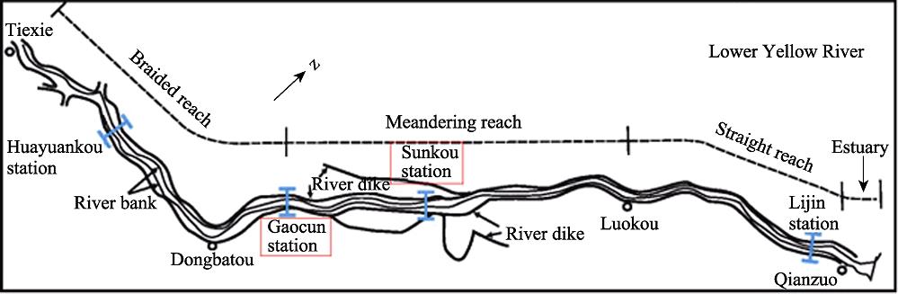
In recent decades, the worldwide frequency of extreme weather events attributed by global warming has brought serious disasters to the international society, and the study predicted the threat will continue to increase in the future. Meanwhile, the Yellow River has always been suffering from frequent devastating floods, droughts, and the consequent channel changes. The Lower Yellow River (LYR) has a length of 786 km and an average slope of 0.12‰ measured from the Taohuayu Valley to the estuary of the Yellow River. In general, this region is divided into four sub-reaches: the braided Huayuankou-Gaocun reach, the transitional Gaocun-Sunkou reach, Sunkou-Aishan reach, and the meandering Aishan-Lijin reach. Hyper-concentrated flows frequently occur in the Lower Yellow River due to the serious soil erosion on the Loess Plateau. Many dams were constructed along the mainstream and have aroused the drastic changes in river regime over time. Particularly zero flow conditions (Yang et al., 2010) so called “hump phenomenon” occurred in the Lower Yellow River as a result of the climate variations and increasing water consumption. As shown the Gaocun-Sunkou reach in Figure 1, the flow capacity here was much less than both up-down streams, and Gaocun station went through a sharp rise in the elevation of river bed in 1994 to 2002 (Deng et al., 2015; Guo et al., 2012). For contributing more on the issues, the channel geometry data (Table 1) along the Gaocun station downwards are applied as the base data for examining the stochastic models proposed and further investigating the dynamic evolution of hydraulic geometries over a long term in the sections below as we will see.

We estimate the unknown parameters set of stochastic discharge in the first place, and then deal with the ones of stochastic hydraulic geometries. For validating the SDEs, time range is assigned to be [1952, 2013], time interval is 1, iterative step is arranged as 1/12. A problem occurred in the application of the nonparametric estimate procedure that initial value could significantly affect the optimization result due to the use of “fmincon” function. Then our solution out of many attempts is to perform multiple calculations; every single process is initialized with the average of the previous results, thus greatly reducing the importance of initial value. After each calculation at 5,000 runs with 1,000 computer-generated sample datasets, the parameter estimation results are well obtained (Tables 2-7). Additionally, we also evaluate the deterministic Eqs.(6) with a least square fit as the control groups for ease of comparative study.

With the estimated parameters, the dynamic probabilities of bankfull discharge and hydraulic geometries can be approximated by repeated computations (over 10,000 runs) on the SDEs. For the jump-diffusion cases, based on maximizing the relevance of stochastic average (the mean value of the computation results for every year) and measurements from a given stimulus intensity, the optimal jump moments can be estimated (Figures 2-4). The following reveals the calculated probability evolution results.

3.3.1 Model-1

It can be seen from Figure 2 that, by adding white noise, SDEs broaden and improve the descriptive power of deterministic equations in the probability distribution ways. Obviously, the stochastic average of bankfull discharge is much more approximate to the discrete data, and all the moves between the probabilistic distributions of hydraulic geometry with measurements have the general tendency in common, which testify a degree of the validity of white-noise SDEs for describing the dynamic evolution tendency. However, the fact is, the real fluctuation characteristics of hydraulic geometry are not well in control, the simulated average trend beginning around 1997 deviates much from the measurements; seemingly, as expected, stochastic processes driven by Gaussian white noises have excessive continuities, not enough breaking information, so that some local changes are over-predicted or under-predicted severely, which undoubtedly reduces their effectiveness for predicting the possibility of bifurcation’s occurrence. That reminds us the complexity of the dynamic river system and the limitation of making Gaussian white noise as the only random disturbances. Just like absence of enough centrifugal force would lead car to skid off the track, obviously SDEs-(8) requires additional reinforcement.

3.3.2 Model-2

Jump-diffusion model was first introduced by Merton (1976) who solved the option prices combining with Gaussian white noise and lognormally distributed Poisson jumps. Considering the sudden heavy changes in meteorological conditions or artificial disturbances could bring random impulse excitation to bankfull channel geometries, and that all the occurrence, duration and magnitude of such processes are random, thus we built a jump-diffusion model SDEs-Eqs. (10). In this section, the continuous change of bankfull geometries are regarded as the combination of geometric Brownian motion and Poisson jump-diffusion motion, which describe the continuous processes and the unexpected destruction of continuities, respectively. See Figure 3a, the variation of discharge by taking the Model-2 approach successfully limits the excessive expressiveness of white noises and improves the simulation effectiveness on the whole. Compared with Figures 2b-2e, Figures 3b-3e show a positive development that the plane probability stability zones are turned from smooth and thick into more uneven and exquisite form, meanwhile the increased volatility molds the average trends into more real representation of the hydraulic geometry variations. The phenomenon prove that the simulated jump terms have succeeded in detecting sudden events, Poisson SDEs is definitely an important extension to the theory of stochastic processes and could highly enhance the capability of simulation in some cases. The only downside here is that local excessive transiliences are completely beyond the effective interval solutions. In some moments, hydraulic geometry with UP or DOWN lead to overlarger UP or DOWN, or oversharp reversal reaction. Obviously, sometimes nonlinearity dominates in the dynamics.

3.3.3 Model-3

The research of fBm can be traced back to the early 1940s. Mandelbrot and Aizenman (1979) named it and promoted the fractal family. In recent years, fBm has been found in applications to natural and engineering sciences, for example, turbulence in hydraulics. Thus, we established a jump-diffusion SDEs-Eqs.(13) driven by fBm to further explore the nonlinear characteristics of bankfull channel geometry. Overall, we can see similar performances with Figure 3 in the bankfull discharge case, and meanwhile Figures 4b-4e perform better than Figures 3b-3e, in particular, the width and velocity process with the Hurst parameters in the range of 0 to 0.5 are severely negatively correlated, the time series for each are long-term switched between high and low values in adjacent pairs, which is well consistent with actual situation. While for the slope and depth case, the fractional model is similar to the jump model in the ways that some local jump events are correctly captured while others are not. Also, a noteworthy point is that some outlier points are still not incorporated in the core of probabilistic regions, there could be a chance of gradual improvement by advancing Poisson noises on the basis of fractional white noise. Considering Poisson Jump may be much more complicated than it appears, we believe adding zoom factor in jump intensity or jump frequency, or substituting for the mutually independent noises with correlated noises could really be alternative options to consider in the future work. In summary, the description of the SDEs behaviors is investigated with satisfactory outcomes.

Through the consistent procedure running based on SDEs, the variation of bankfull channel geometries are demonstrated to be characterized by nonlinearity, non-stationary, and abruptness. Here deterministic equilibrium curves are converted into probabilistic distribution zone, in which the significant interval and the average trend could greatly determine the research value for river management. The implementation of SDEs provides such kind of important supplement that we move on to conduct a comparable study of the different models in a quantitative way. Obviously, in case that exterior integral styles permitted, it will be satisfying to choose a model with the larger of effective probability (the average occurring probability of discrete measurements in the distributions) and the smaller of effective probability stability thickness (the interior limit range), and also the smaller of the relative error between stochastic average and measurements. Considering the great significance of the above factors for the investigation and comparison, we describe below their time-varying processes (Figures 5-6), and in consistent with Figures 2-4, we give targeted suggestions for each hydraulic geometry relation in the following parts.

(1) Slope. Figures (2-4)b show that jump-diffusion models could strongly help to improve the capacity for controlling systemic slope changes, and simple Gaussian white noise model should undoubtedly be abandoned. Meanwhile judging by Figures (5-6)a, victory belongs to fractional model due to its overall advantage in effective stability thickness and effective probability, though the Model-2 enjoys a bit advantage over relative error of dataset.

(2) Width. Similar to the slope case, according to Figures (2-4)c, intuitively, we can find the significant improvement of jump-diffusion models over simple white noise model. The fractional approach has the advantage of having little relative error, and better performance in simulating the fluctuation of stochastic average.

(3) Depth. Different to the above cases, Figures (2-4)d show the slight rising effect of fractional term in describing the dynamic changes on the basis of Poisson jump. According to the performances in the effective probabilistic zone and relative data error in Figures (5-6)c, it seems Poisson jump could take effect well only under the linear Gaussian circumstances. In other words, dynamic depth can thus be proven to be highly continuous, stable, and be affected linearly by unexpected stochastic events.

(4) Velocity. In this case, Figures (2-4)e and Figures (5-6)d show that fractional SDEs is superior to Poisson jump model, especially in the fluctuation of the simulation results, effective probability properties and relative error (δ). Obviously, the performance of fractional model is charmed and convinced.

In short, fractional jump-diffusion model has best applicability in simulating the slope, width, and velocity changes, the simple jump-diffusion model is good enough for exploring depth.

In a certain sense river is alive, like a man, bankfull channel geometries constitute the primary organ of river body. Fundamentally, discharge plays the role of drivers and sustainers of diversified river landscape. And in many cases, there are a number of reasons to explain the nonlinearity of hydraulic geometry relations, such as the presence of gravel bars, the variability of hydraulic geometry of riffles, or an abrupt change in the resistance to flow (Navratil and Albert, 2010), while the assessment of system stability is always a very necessary task in understanding river. According to the literature, some excellent tools could be used to describe it, for example, the riverbed stability indices (Z_w) by Zhang (1995) (Eq. 24a) has the ability to help to distinguish different river patterns including braiding (Z_w<5), anabranching (or transitioning) (5<Z_w<15) and meandering type (Z_w>15). And similarly, hydraulic width/depth ratio (ζ) (Eq. 24b) and stream power (Ω) (Eq. 24c) can be regarded as the characteristic quantities that represent erosion rate and flow intensity in a river. Thus, from the foregoing research results, we perform statistical computations on the dynamic probability processes of Z_w, ζ and Ω observed from the Gaocun station downward with all individual hydraulic geometry variables in their fractional stochastic definitions being already calculated in former sections, as is shown in Figure 7.

It can be seen from Figure 7a that riverbed stability indices began to fall starting from 1990, whose stochastic average almost passed the Z_w=5 braiding threshold during the following period, then until the year 2000 it was gradually strengthened and returned to the transitional zone (5<Z_w<15). Meanwhile, Gaocun station was powered by slowly increased flow intensity (Figure 7c), and dominated more by incision than by widening erosion (Figure 7b) after 2000. The reason, according to the literature, is the running and application of the upstream Xiaolangdi Reservoir spared long-suffering low flow and sediment load burden in Lower Yellow river, which is consistent with the hump phenomenon that was proven to be negatively correlated with the flow discharge level by Guo et al. (2012). The above figures demonstrate that the trough of river stability around 1999 has been saved; the sensitive fluctuation of probability thickness with average trendline reminds us of needs that raise the level of river evolution alert in Lower Yellow River in the future. Moreover, this also sees the ascendancy of SDEs, considering the discrete data calculated on the basis of measurement do not completely reflect the changing reality, such as in ζ around 2000. That means the measurements of the individual hydraulic geometry variables cannot help us to exactly grasp the dynamic characteristics of river system, yet hydraulic width/depth ratio (ζ) as an example expressed by the proposed stochastic method could work in the conditions of only small amount data of flood season’s discharge and suspended sediment concentration. Calculations of correlation coefficients of stochastic average Z_w , ζ and Ω with bankfull discharge (Q) (Table 8) lead us to believe that discharge-dominated Lower Yellow River can be described better with a stochastic state space represented by Ω. Fresh information collected in Lower Yellow River show that the region is suffering from a combination of water and soil conservation, upstream reservoir regulation, increasing water usage and climatic change after 2013, the water-sediment amount coming into the mainstream continue decreasing sharply. The demand for sustainable and stable development of the Yellow River Plain requires us to handle seriously the new situation of enhanced channel capacity of water flow and more appearance of medium-small discharge. Long-term relevant influences need to be measured, identified, and assessed by systematical and quantitative methods. This study is of great theoretical and practical significance.

This paper considered the bankfull channel geometry problem for a stochastic time-varying state space of multi-input multi-output river system by involving random noise factors in the stochastic differential equations. Three different models that combined the Gaussian white noise, Fractional white noise, Poisson noise were evaluated respectively in the Gaocun-Sunkou reach of the Lower Yellow River to investigate the evolution of probability distribution of bankfull channel geometries here over time. Results show that this procedure effectively extends the traditional deterministic equations into the controllable probabilistic stability forms, successfully improves the understanding of systemic river evolution under limited data conditions, and, contributes much to river management and the utilization of the earth’s surface resources. Future research will continue to receive new authentication and become more perfect by avoiding the use of over-simplified noise terms.

References

[1] Handbook of Financial Econometrics: Tools and Techniques. Elsevier(2009).
[2] Rate of floodplain reworking in response to increasing storm-induced floods, Squamish River, south-western British Columbia, Canada. Earth Surface Processes & Landforms, 36, 872-884(2011).
[3] The pricing of options and corporate liabilities. Journal of Political Economy, 81, 637-654(1973).
[4] A nonlinear model for river meandering. Water Resources Research, 45, 546-550(2009).
[5] Approximation of jump diffusions in finance and economics. Research Paper, 29, 283-312(2006).
[6] Convergence and stability analysis for implicit simulations of stochastic differential equations with random jump magnitudes. Discrete and Continuous Dynamical Systems: Series B (DCDS-B), 9, 47-64(2017).
[7] et alAn empirical comparison of alternative models of the short-term interest rate. Journal of Finance, 47, 1209-1227(1992).
[8] Stochastic analysis of the Fractional Brownian Motion. Potential Analysis, 10, 177-214(1999).
[9] Study on particularity of hump reach evolution in Lower Yellow River. Yellow River, 37, 28-31(2015).
[10] Monte Carlo Methods in Financial Engineering. Springer(2004).
[11] Catastrophe theory as a model for change in fluvial systems. Adjustments of the Fluvial System, 13-32(1979).
[12] et alFormation and development of hump reach in Lower Yellow River. Journal of Sediment Research, 38-42(2012).
[13] et alGlobal warming in the twenty-first century: An alternative scenario. Proceedings of the National Academy of Sciences of the United States of America, 97, 9875-9880(2000).
[14] et alCoupled geomorphic and habitat response to a flood pulse revealed by remote sensing. Ecohydrology, 10(2017).
[15] A history of the systems approach in geomorphology. Géomorphologie Relief Processus Environnement, 13, 145-158(2007).
[16] Spatial process simulation. Springer International Publishing, Cham, 369-404(2015).
[17] et alOn the self-similar nature of Ethernet traffic (extended version). Acm Sigcomm Computer Communication Review, 25, 202-213(1995).
[18] Nonlinear forecasting using nonparametric transfer function models. Wseas Transactions on Business & Economics, 157, 151-164(2009).
[19] Spatial width oscillations in meandering rivers at equilibrium. Water Resources Research, 48, 375-390(2012).
[20] Fractals: Form, chance, and dimension. Leonardo, 32, 65-66(1979).
[21] A stochastic approach for the description of the water balance dynamics in a river basin. Hydrology & Earth System Sciences, 12, 1189-1200(2008).
[22] Option pricing when underlying stock returns are discontinuous. Working Papers, 3, 125-144(1976).
[23] Effects of river flow scaling properties on riparian width and vegetation biomass. Water Resources Research, 43, W12406(2007).
[24] Non-linearity of reach hydraulic geometry relations. Journal of Hydrology, 388, 280-290(2010).
[25] Nonlinearity and unsteadiness in river meandering: A review of progress in theory and modelling. Earth Surface Processes & Landforms, 36, 20-38(2011).
[26] Maximum likelihood estimation of the double exponential jump-diffusion process. Annals of Finance, 3, 487-507(2007).
[27] Theory of stochastic differential equations with jumps and applications: Mathematical and analytical techniques with applications to engineering. Springer Science &Business Media(2006).
[28] Likelihood methods for diffusions with jumps, Statistical inference in stochastic processes. Marcel Dekker Incorporated, 67-105(1991).
[29] Density estimation for statistics and data analysis. Technometrics, 29, 495(1987).
[30] A nonparametric model of term structure dynamics and the market price of interest rate risk. Journal of Finance, 52, 1973-2002(1997).
[31] Modeling the impact of river damming on riparian vegetation. Journal of Hydrology, 396, 302-312(2011).
[32] Stochastic particle based models for suspended particle movement in surface flows. International Journal of Sediment Research, 29, 195-207(2014).
[33] River Dynamics and Integrated River Management. Berlin Heidelberg:Springer(2015).
[34] Periodic transfer function-noise model for forecasting. Journal of Hydrologic Engineering, 10, 353-362(2005).
[35] Relative scales of time and effectiveness of climate in watershed geomorphology. Earth Surface Processes and Landforms, 3, 189-208(1978).
[36] et alResponse of bankfull discharge to discharge and sediment load in the Lower Yellow River. Geomorphology, 100, 366-376(2008).
[37] et alResponse of reach-scale bankfull channel geometry to the altered flow and sediment regime in the lower Yellow River. Geomorphology, 213, 255-265(2014).
[38] Hydraulic geometry and minimum rate of energy dissipation. Water Resources Research, 17, 1014-1018(1981).
[39] et alA spatial assessment of hydrologic alteration caused by dam construction in the middle and lower Yellow River, China. Hydrological Processes, 22, 3829-3843(2010).
[40] New methods for simulation of fractional brownian motion. Journal of Computational Physics, 127, 66-72(1996).
[41] The study of the law of similarity for models of flood flows of the lower reach of the Yellow River. Beijing: Tsinghua University(1995).
Xiaolong SONG, Deyu ZHONG, Guangqian WANG. Simulation on the stochastic evolution of hydraulic geometry relationships with the stochastic changing bankfull discharges in the Lower Yellow River[J]. Journal of Geographical Sciences, 2020, 30(5): 843
Download Citation