
Qi Geng, Ka-Di Zhu. Discrepancy between transmission spectrum splitting and eigenvalue splitting: a reexamination on exceptional point-based sensors[J]. Photonics Research, 2021, 9(8): 1645
- Photonics Research
- Vol. 9, Issue 8, 1645 (2021)
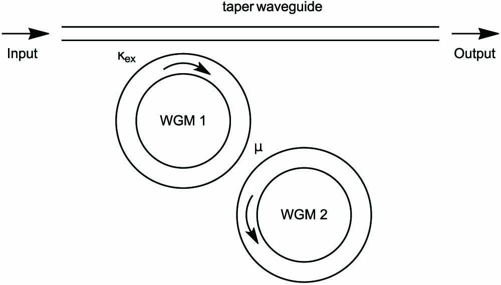
Fig. 1. Schematic of the system consisting of two coupled whispering-gallery microcavities. We have not explicitly drawn the taper in the figure.
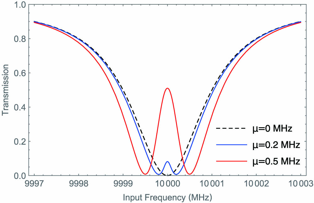
Fig. 2. Spectrum of two coupled cavities, which has a splitting similar to EIT. The parameters are w 1 = w 2 = 10 GHz κ 1 / 2 = 1 MHz κ 2 / 2 = 0.1 MHz κ ex = κ 1 / 2 μ = 0 , 0.2 , 0.5 MHz P ( w ) = 0 μ = 0 λ 1 = 10 , 000 − i λ 2 = 10 , 000 − 0.1 i r 1 = 10 , 000 r 2 = 10 , 000 − 0.1 i μ = 0.2 M H z λ 1 = 10 , 000 − 0.15 i λ 2 = 10 , 000 − 0.95 i r 1 = 9999.81 − 0.05 i r 2 = 10 , 000.19 − 0.05 i μ = 0.5 MHz λ 1 = 9999.78 − 0.55 i λ 2 = 10 , 000.22 − 0.55 i r 1 = 9999.50 − 0.05 i r 2 = 10 , 000.50 − 0.05 i
Fig. 3. Re ( Δ λ ) Re ( Δ r ) P ( w ) = 0 Δ W Δ W Re ( Δ r ) μ Re ( Δ λ ) ≈ Re ( Δ r ) 2 .
Fig. 4. Transmission rate in case w 1 ≠ w 2 w 1 = 10 , 000 MHz w 2 = 10 , 000.1 MHz κ 1 / 2 = 1 MHz κ 2 / 2 = 0.1 MHz μ = 0.3 MHz
Fig. 5. Transmission rate for different Δ μ w 1 = w 2 = 10 GHz κ 1 / 2 = κ 2 / 2 = κ ex / 2 = 1 MHz μ 0 = 1 MHz μ = μ 0 + Δ μ Δ μ = 0 , 0.1 , 0.2 MHz Δ μ Δ W 2 Δ W 2 = 8 Δ μ Δ μ 10 ).

Set citation alerts for the article
Please enter your email address
© Copyright 2018-2021 | Chinese Laser Press. All Rights Reserved 沪ICP备15018463号-20