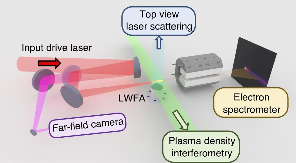
Fig. 1. Illustration of the experimental setup (not to scale). The primary laser focus was aligned to the front edge of a supersonic gas jet emitted from a 15 mm diameter nozzle positioned 10 mm below the laser pulse propagation axis. The input laser energy was measured by integrating the signal on a near-field camera before the compressor, which was cross-calibrated with an energy meter and adjusted for the 60% compressor throughput. The scattered laser signal was observed from above by an optical camera, and the plasma channel electron density profile was measured using interferometry with a transverse short-pulse probe laser. The small () transmission of the focusing laser pulse through a dielectric mirror was directed onto a CCD camera to obtain an on-shot far-field image. Electron beams from the LWFA were deflected by a magnetic dipole onto two Lanex screens (only the first is shown here), which were used to determine the electron spectrum in the range of GeV.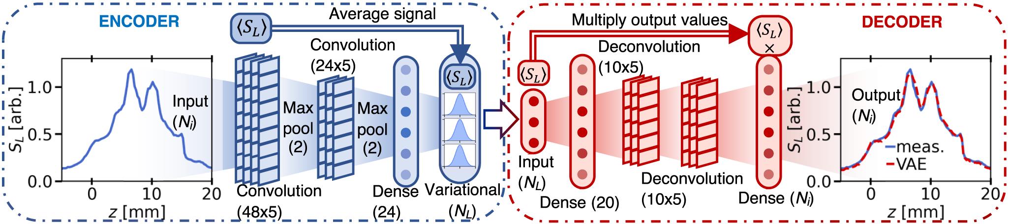

Fig. 2. Variational autoencoder (VAE) architecture for determining the latent space representation of the diagnostics. The type and dimension of each layer are indicated in the labels. The inset plots show an example laser scattering signal and the approximation returned by the VAE. The input (and output) size is equal to the data binning of the results for each individual diagnostic. Max pooling was used at the output of each convolution layer, which combined neighbouring output pairs and returned only the maximum of each pair. The average signal, in this case , was passed as an additional latent space parameter for the encoder and was used to scale the output of the decoder. The autoencoder structure was the same for each diagnostic, except for the size of the latent space.

Fig. 3. Diagram of the translator network architecture. Shown in the inset is an example measurement from the experimental data (black), with the mean prediction of the LWFA model ensemble (red) and individual model predictions (pink).

Fig. 4. (a) Measured electron spectra and reproduced electron spectra using (b) the trained variational autoencoder and (c) the mean prediction of the ensemble of the LWFA models. The individual shots are sorted by cut-off energy, determined as the highest energy for which the spectra exceed a threshold value.

Fig. 5. Individual shots selected at equally spaced intervals of the sorted shot index from Figure 4. The measured spectra (black) are shown alongside the predictions of each LWFA model from the trained ensemble (red) and an individual spectrum measurement closest to the median of the training data (blue). The sorted shot index is shown in the top right of each panel.

Fig. 6. Relative influence of the translator VNN input parameters on the predicted electron spectra. Each parameter is set to the mean value of the training dataset and then varied over standard deviations in 11 steps, with the variation in the spectrum quantified by the average RMS change to the spectrum. The nth latent space parameters for the scattering and density profile encoders are labelled and , respectively. Here, and are proportional to the average laser scattering signal and plasma electron density, respectively.

Fig. 7. The model predicted effect of varying the laser energy on (a) the predicted electron spectra and (b) the total electron beam charge. The data for each shot in the training data (red) are shown in (b), overlaid from the values calculated from the predicted spectra of the LWFA model (black points) with a linear fit (black dashed line).

Fig. 8. The effect of changing on (a) the electron density profile and (b) the predicted electron spectrum. All other latent space parameters are kept fixed at zero (i.e., their average values from the training dataset), while is varied over the range of standard deviations in the training dataset.

Fig. 9. The effect of changing on (a) the laser scattering profile and (b) the predicted electron spectrum. All other latent space parameters are kept fixed at zero (i.e., their average values from the training dataset), while is varied over the range of standard deviations in the training dataset.

Table 1. Summary of autoencoder parameters used for each diagnostic and for the translator model.