
M. J. V. Streeter, C. Colgan, C. C. Cobo, C. Arran, E. E. Los, R. Watt, N. Bourgeois, L. Calvin, J. Carderelli, N. Cavanagh, S. J. D. Dann, R. Fitzgarrald, E. Gerstmayr, A. S. Joglekar, B. Kettle, P. Mckenna, C. D. Murphy, Z. Najmudin, P. Parsons, Q. Qian, P. P. Rajeev, C. P. Ridgers, D. R. Symes, A. G. R. Thomas, G. Sarri, S. P. D. Mangles, "Laser wakefield accelerator modelling with variational neural networks," High Power Laser Sci. Eng. 11, 010000e9 (2023)
- High Power Laser Science and Engineering
- Vol. 11, Issue 1, 010000e9 (2023)
Abstract
1 Introduction
Laser wakefield accelerators (LWFAs) generate multi-GeV electron beams from cm-scale plasma channels using approximately 100 TW laser pulses[1–6]. The extreme acceleration gradients of LWFAs, coupled with their relative accessibility, have led to widespread research and pursuit of several applications, such as compact light sources[7–10], generation of bright
In LWFAs, the non-linear laser pulse evolution[18,19] and its effect on the injection and acceleration processes[20–23] are highly sensitive to the initial conditions and can lead to significant shot-to-shot variation of the electron beam properties[24,25]. Recent work on high-stability laser systems and plasma sources has demonstrated improved stability, with the observation of few-percent variation in the electron beam energy and charge over 24 hours of continuous operation[26]. Long-term high-repetition rate operation has opened up the possibility of using machine learning techniques to model the sources of electron beam variation and to use closed-loop algorithms to optimise performance[26–31].
For applications such as the study of the radiation reaction, knowledge of the pre-interaction electron beam properties is required to make precise measurements of any changes of these properties and thereby infer the validity of theoretical models[32–34]. The destructive nature of the measurements necessitates predictable LWFA performance through one of the following: improved stability; preserving part of the spectrum as a reference[33]; or by developing models capable of producing the electron beam properties from a given shot. In general, the ability to make predictions of the outputs from plasma accelerators will be advantageous to many of their applications.
Sign up for High Power Laser Science and Engineering TOC. Get the latest issue of High Power Laser Science and Engineering delivered right to you!Sign up now
Previous work in developing machine learning models for LWFAs has demonstrated the prediction of scalar metrics of the electron beam, such as total charge or peak energy[29–31,35]. However, many applications will require the prediction of vector properties, such as the spectrum or the longitudinal phase space, for which neural networks provide a convenient framework. A densely connected neural network (DNN) is made of densely connected layers, in which every input is the weighted sum of all of the outputs of the previous layer, with the individual weights as free parameters of the model. A non-linear activation function (e.g., a sigmoid function) then takes the weighted sum plus a bias value (another free model parameter) as its argument and returns an output value. An alternative to deeply connected layers is a convolutional layer, which performs convolutions between the input vector and a set of kernels. Networks using these layers, known as convolutional neural networks (CNNs), have been shown to be better suitable for learning meaningful features from natural signals[36]. Further improvement to the predictive power of neural networks has been seen when including stochasticity in the outputs of individual nodes, in an architecture known as a variational neural network (VNN)[37].
In conventional accelerators, Emma et al.[38] demonstrated training of a DNN to produce synthetic diagnostic outputs that matched the measured outputs for a new unseen dataset. CNNs have been used to predict X-ray properties from the post-undulator electron beam spectrum[39], while ensembles of DNNs have also been used to predict the electron beam longitudinal phase space and current profile from non-destructive bending radiation measurements[40]. In this work, we report on the training of an ensemble of VNNs to model the LWFA-generated electron spectrum using secondary diagnostics of the laser and plasma conditions. The LWFA ensemble was trained using a subset of experimental measurements of the electron spectrum with the remainder used for model validation. Each individual VNN in the ensemble was trained with a different subset of the training data, so that the ensemble provided both a mean prediction and an estimate of its uncertainty. The model also reveals the extent to which the measurements obtained from the available diagnostics are predictive of the accelerator performance, and which parameters have the strongest influence.
2 Experimental methods and results
The experiment was performed using the Gemini laser system at the Central Laser Facility in the UK (see Figure 1 for details). Laser pulses with an energy of
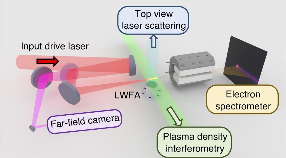
Figure 1.Illustration of the experimental setup (not to scale). The primary laser focus was aligned to the front edge of a supersonic gas jet emitted from a 15 mm diameter nozzle positioned 10 mm below the laser pulse propagation axis. The input laser energy was measured by integrating the signal on a near-field camera before the compressor, which was cross-calibrated with an energy meter and adjusted for the 60% compressor throughput. The scattered laser signal was observed from above by an optical camera, and the plasma channel electron density profile was measured using interferometry with a transverse short-pulse probe laser. The small ( ) transmission of the focusing laser pulse through a dielectric mirror was directed onto a CCD camera to obtain an on-shot far-field image. Electron beams from the LWFA were deflected by a magnetic dipole onto two Lanex screens (only the first is shown here), which were used to determine the electron spectrum in the range of
  GeV.
GeV.
The LWFA-generated electron energy spectrum
The experimental results for this analysis were taken from an investigation of the radiation reaction, in which a second counter-propagating laser pulse is used to collide with the LWFA electron beam. For training and validating our predictive tool, we wish to only use shots where the laser pulse did not significantly overlap with the electron beam, so that the electron spectrum was not affected. For successful collisions, a gamma-beam was generated via the inverse Compton scattering interaction and was diagnosed spatially with a CsI scintillator array[16] imaged onto a
Due to the shot-to-shot variation in the electron beam position, most shots did not result in a significant collision, providing a large number of null shots for model training and testing. The brightness of the signal on the gamma detector was used to provide an approximate metric of the collision intensity. The 99.99th percentile pixel value of the background subtracted CCD image was taken as the peak of the gamma signal
3 Neural network architecture and training
The measurements of
![]()
Figure 2.Variational autoencoder (VAE) architecture for determining the latent space representation of the diagnostics. The type and dimension of each layer are indicated in the labels. The inset plots show an example laser scattering signal  and the approximation returned by the VAE. The input (and output) size
  is equal to the data binning of the results for each individual diagnostic. Max pooling was used at the output of each convolution layer, which combined neighbouring output pairs and returned only the maximum of each pair. The average signal, in this case
  , was passed as an additional latent space parameter for the encoder and was used to scale the output of the decoder. The autoencoder structure was the same for each diagnostic, except for the size of the latent space.
The trained encoders for
![]()
Figure 3.Diagram of the translator network architecture. Shown in the inset is an example measurement from the experimental data (black), with the mean prediction of the LWFA model ensemble (red) and individual model predictions (pink).
For the variational layers, two parameters are calculated for each node that represent the expectation value
| Model | Validation | |||
|---|---|---|---|---|
| Density profile | 310 | 4+1 | ||
| Scattering profile | 100 | 5+1 | ||
| Electron spectra | 200 | 4+1 | ||
| LWFA single | 18 | 5 | ||
| LWFA ensemble | 18 | 5 |
Table 1. Summary of autoencoder parameters used for each diagnostic and for the translator model.
The training loss function used was as follows[45]:
For the diagnostic VAEs, the number of latent parameters was chosen to be the minimum that gave high-fidelity reconstructions, with the
The translator is a DNN with a variational last layer. The translator VNN architecture (number of nodes and number of layers) and the value of
In order to quantify the uncertainty in the model predictions, 100 translator VNNs were trained, each using randomly selected 50% samples of the training dataset. The prediction of each of these models can then be used to obtain an average prediction, while the variation between model predictions is indicative of the random uncertainty and the finite size of the training data. In particular, the random sub-sampling affects the predictive quality in regions where the training data are sparse, typically at the extremes of the input parameters, resulting in a larger uncertainty in those regions.
The parameters for the trained VAEs and translator networks are summarised in Table 1. Each autoencoder was trained for 1000 iterations with a batch size of 64. The translator network was trained in three stages with 200, 400 and 300 iterations performed at 10, 4 and 1 times the final
4 LWFA prediction results
The measured electron spectra from the validation dataset are shown in Figure 4(a), along with the reconstructions by the electron spectra VAE (Figure 4(b)) and the average of the LWFA model ensemble predictions (Figure 4(c) ). The electron spectra VAE had an MSE of 0.011, and shows good qualitative and quantitative reproduction of the measured electron spectra. This indicates that the five parameters of the latent space, in combination with the structures learnt by the decoder, are sufficient to accurately generate the set of observations from the validation dataset. In other words, the five latent parameters are sufficient to generate the full variability of electron beams for this experimental setup. The question is then whether the secondary diagnostics are sufficient to determine the correct latent variables for each shot and thereby give an accurate prediction of the electron spectrum. The mean prediction of the LWFA model ensemble had an MSE of 0.057 and shows a similar trend in cut-off energy to the data, except for the few high- and low-energy outliers. By comparison, a naive prediction that all measured spectra are equal to the average spectrum from the training dataset gives an MSE value of 0.11, indicating that the LWFA model has a significant predictive capability.
![]()
Figure 4.(a) Measured electron spectra and reproduced electron spectra using (b) the trained variational autoencoder and (c) the mean prediction of the ensemble of the LWFA models. The individual shots are sorted by cut-off energy, determined as the highest energy for which the spectra exceed a threshold value.
Individual predictions of each model of the LWFA ensemble, along with the corresponding measured electron spectra, are shown in Figure 5. The variation in model predictions for a given shot is indicative of the uncertainty, due to the random sub-sampling of the training data and the stochastic training process. For a large region of the parameter space, the LWFA model predictions show a good agreement with the measurements, with large discrepancies occurring for the outliers in terms of cut-off energy. These shots also exhibit the largest variation in predictions between individual models within the ensemble. The total electron beam energy is reasonably accurately predicted, with relative RMS error of 12% for the entire validation dataset, compared to the relative beam energy RMS variation of 30%.
![]()
Figure 5.Individual shots selected at equally spaced intervals of the sorted shot index from Figure 4. The measured spectra (black) are shown alongside the predictions of each LWFA model from the trained ensemble (red) and an individual spectrum measurement closest to the median of the training data (blue). The sorted shot index is shown in the top right of each panel.
The relative influence of each input parameter on the LWFA model can be seen by varying each one in turn and measuring the effect on the resultant spectrum, as shown in Figure 6. The plasma density parameters have a relatively modest effect on the electron spectrum, indicating that the shot-to-shot variation of the plasma density profile is not the dominant contributor to the electron spectrum variation. Variations of the laser energy and the scattering profile are more significant, having the greatest effect on the generated electron spectra. The spatio-temporal distribution of the laser pulse is only indirectly diagnosed from the far-field diagnostic and the effect on the scattering profile, and is known to have a large influence on the accelerated electrons[26,28,29]. Including additional laser diagnostics, such as measurement of the spatial phase profile[26,30], should enable higher fidelity predictions.
![]()
Figure 6.Relative influence of the translator VNN input parameters on the predicted electron spectra. Each parameter is set to the mean value of the training dataset and then varied over  standard deviations in 11 steps, with the variation in the spectrum quantified by the average RMS change to the spectrum. The
  and
and  , respectively. Here,
  and
and  are proportional to the average laser scattering signal and plasma electron density, respectively.
Although many of the input parameters are not straightforward to interpret physically, that is, those that are the latent space of the autoencoders, the laser energy is a physically important parameter in LWFAs. In practice, the inputs for the LWFA models are not independent of one another, as characterised by calculating the Pearson correlation coefficients for the training dataset. This reveals relatively strong correlations between the laser energy and several other parameters, especially
![]()
Figure 7.The model predicted effect of varying the laser energy on (a) the predicted electron spectra and (b) the total electron beam charge. The data for each shot in the training data (red) are shown in (b), overlaid from the values calculated from the predicted spectra of the LWFA model (black points) with a linear fit (black dashed line).
The scaling parameters
![]()
Figure 8.The effect of changing  on (a) the electron density profile and (b) the predicted electron spectrum. All other latent space parameters are kept fixed at zero (i.e., their average values from the training dataset), while
  is varied over the range of
  standard deviations in the training dataset.
The other latent parameters generated by the VAEs do not have straightforward physical interpretations and only have meaning in combination with the trained encoders. In order to gain some insight into their physical meaning, the effect of changing each parameter can be observed on the corresponding diagnostic output, as well as on the predicted electron spectrum. An example is shown in Figure 9, where the effect of varying
![]()
Figure 9.The effect of changing  on (a) the laser scattering profile and (b) the predicted electron spectrum. All other latent space parameters are kept fixed at zero (i.e., their average values from the training dataset), while
  is varied over the range of
  standard deviations in the training dataset.
Figure 9(a) shows that positive
5 Conclusion
In conclusion, we have constructed and trained a predictive model for an LWFA that is capable of predicting the electron spectrum for a given shot, based on secondary diagnostics of the laser and plasma conditions. The model is constructed from separately trained variational convolutional autoencoders, with a VNN used to map a reduced parameter set to the latent space of an electron spectra decoder. An ensemble of models was trained on subsets of the training data, with the range of model predictions providing an estimate of the uncertainty. The predictive model ensemble performs better than the naive assumption that the electron spectrum is constant, and so has utility in estimating the electron spectrum in the case of destructive processes, such as a radiation reaction. The model fidelity is most likely limited by the lack of on-shot spatio-temporal information about the laser pulse, which is known to have a strong influence on the accelerated electron beam[26]. It is expected that this technique can be improved by including additional diagnostics of the laser spatial and spectral phase, and by increasing the size of the training dataset, especially for reducing the prediction error for the outliers. Further diagnostics of the laser–plasma interaction, such as spectrally resolving the scattering signal, may also provide additional information to improve the prediction accuracy. Neural networks of this kind could be an important tool for understanding the performance sensitivities of plasma accelerators, and also in providing synthetic diagnostics for applications of their electron beams and secondary sources.
References
[1] W. P. Leemans, B. Nagler, A. J. Gonsalves, C. Tóth, K. Nakamura, C. G. R. Geddes, E. Esarey, C. B. Schroeder, S. M. Hooker. Nat. Phys., 2, 696(2006).
[2] S. Kneip, S. R. Nagel, S. F. Martins, S. P. D. Mangles, C. Bellei, O. Chekhlov, R. J. Clarke, N. Delerue, E. J. Divall, G. Doucas, K. Ertel, F. Fiuza, R. Fonseca, P. Foster, S. J. Hawkes, C. J. Hooker, K. Krushelnick, W. B. Mori, C. A. J. Palmer, K. T. Phuoc, P. P. Rajeev, J. Schreiber, M. J. V. Streeter, D. Urner, J. Vieira, L. O. Silva, Z. Najmudin. Phys. Rev. Lett., 103, 035002(2009).
[3] C. E. Clayton, J. E. Ralph, F. Albert, R. A. Fonseca, S. H. Glenzer, C. Joshi, W. Lu, K. A. Marsh, S. F. Martins, W. B. Mori, A. Pak, F. S. Tsung, B. B. Pollock, J. S. Ross, L. O. Silva, D. H. Froula. Phys. Rev. Lett., 105, 105003(2010).
[4] X. Wang, R. Zgadzaj, N. Fazel, Z. Li, S. A. Yi, X. Zhang, W. Henderson, Y.-Y. Chang, R. Korzekwa, H.-E. Tsai, C.-H. Pai, H. Quevedo, G. Dyer, E. Gaul, M. Martinez, A. C. Bernstein, T. Borger, M. Spinks, M. Donovan, V. Khudik, G. Shvets, T. Ditmire, M. C. Downer. Nat. Commun., 4, 1988(2013).
[5] W. P. Leemans, A. J. Gonsalves, H.-S. Mao, K. Nakamura, C. Benedetti, C. B. Schroeder, C. Tóth, J. Daniels, D. E. Mittelberger, S. S. Bulanov, J.-L. Vay, C. G. R. Geddes, E. Esarey. Phys. Rev. Lett., 113, 245002(2014).
[6] A. J. Gonsalves, K. Nakamura, J. Daniels, C. Benedetti, C. Pieronek, T. C. H. de Raadt, S. Steinke, J. H. Bin, S. S. Bulanov, J. van Tilborg, C. G. R. Geddes, C. B. Schroeder, C. T/oth, E. Esarey, K. Swanson, L. Fan-Chiang, G. Bagdasarov, N. Bobrova, V. Gasilov, G. Korn, P. Sasorov, W. P. Leemans. Phys. Rev. Lett., 122, 084801(2019).
[7] H. P. Schlenvoigt, K. Haupt, A. Debus, F. Budde, O. Jäckel, S. Pfotenhauer, H. Schwoerer, E. Rohwer, J. G. Gallacher, E. Brunetti, R. P. Shanks, S. M. Wiggins, D. A. Jaroszynski. Nat. Phys., 4, 130(2008).
[8] A. R. Maier, A. Meseck, S. Reiche, C. B. Schroeder, T. Seggebrock, F. Grüner. Phys. Rev. X, 2, 031019(2012).
[9] F. Albert, A. G. Thomas. Plasma Phys. Control. Fusion, 58, 103001(2016).
[10] W. Wang, K. Feng, L. Ke, C. Yu, Y. Xu, R. Qi, Y. Chen, Z. Qin, Z. Zhang, M. Fang, J. Liu, K. Jiang, H. Wang, C. Wang, X. Yang, F. Wu, Y. Leng, J. Liu, R. Li, Z. Xu. Nature, 595, 516(2021).
[11] G. Sarri, W. Schumaker, A. Di Piazza, M. Vargas, B. Dromey, M. E. Dieckmann, V. Chvykov, A. Maksimchuk, V. Yanovsky, Z. H. He, B. X. Hou, J. A. Nees, A. G. Thomas, C. H. Keitel, M. Zepf, K. Krushelnick. Phys. Rev. Lett., 110, 255002(2013).
[12] G. Sarri, D. J. Corvan, W. Schumaker, J. M. Cole, A. Di Piazza, H. Ahmed, C. Harvey, C. H. Keitel, K. Krushelnick, S. P. D. Mangles, Z. Najmudin, D. Symes, A. G. R. Thomas, M. Yeung, Z. Zhao, M. Zepf. Phys. Rev. Lett., 113, 224801(2014).
[13] B. Cros, P. Muggli. and , (2019).. arXiv:1901.08436
[14] A. G. R. Thomas, C. P. Ridgers, S. S. Bulanov, B. J. Griffin, S. P. D. Mangles. Phys. Rev. X, 2, 041004(2012).
[15] T. G. Blackburn, C. P. Ridgers, J. G. Kirk, A. R. Bell. Phys. Rev. Lett., 112, 015001(2014).
[16] J. M. Cole, K. T. Behm, E. Gerstmayr, T. G. Blackburn, J. C. Wood, C. D. Baird, M. J. Duff, C. Harvey, A. Ilderton, A. S. Joglekar, K. Krushelnick, S. Kuschel, M. Marklund, P. McKenna, C. D. Murphy, K. Poder, C. P. Ridgers, G. M. Samarin, G. Sarri, D. R. Symes, A. G. R. Thomas, J. Warwick, M. Zepf, Z. Najmudin, S. P. D. Mangles. Phys. Rev. X, 8, 011020(2018).
[17] K. Poder, M. Tamburini, G. Sarri, A. Di Piazza, S. Kuschel, C. D. Baird, K. Behm, S. Bohlen, J. M. Cole, D. J. Corvan, M. Duff, E. Gerstmayr, C. H. Keitel, K. Krushelnick, S. P. D. Mangles, P. McKenna, C. D. Murphy, Z. Najmudin, C. P. Ridgers, G. M. Samarin, D. R. Symes, A. G. R. Thomas, J. Warwick, M. Zepf. Phys. Rev. X, 8, 031004(2018).
[18] A. G. R. Thomas, Z. Najmudin, S. P. D. Mangles, C. D. Murphy, A. E. Dangor, C. Kamperidis, K. L. Lancaster, W. B. Mori, P. A. Norreys, W. Rozmus, K. Krushelnick. Phys. Rev. Lett., 98, 095004(2007).
[19] M. J. V. Streeter, S. Kneip, M. S. Bloom, R. A. Bendoyro, O. Chekhlov, A. E. Dangor, A. Döpp, C. J. Hooker, J. Holloway, J. Jiang, N. C. Lopes, H. Nakamura, P. A. Norreys, C. A. J. Palmer, P. P. Rajeev, J. Schreiber, D. R. Symes, M. Wing, S. P. D. Mangles, Z. Najmudin. Phys. Rev. Lett., 120, 254801(2018).
[20] C. Xia, J. Liu, W. Wang, H. Lu, W. Cheng, A. Deng, W. Li, H. Zhang, X. Liang, Y. Leng, X. Lu, C. Wang, J. Wang, K. Nakajima, R. Li, Z. Xu. Phys. Plasmas, 18, 113101(2011).
[21] A. Sävert, S. P. D. Mangles, M. Schnell, E. Siminos, J. M. Cole, M. Leier, M. Reuter, M. B. Schwab, M. Möller, K. Poder, O. Jäckel, G. G. Paulus, C. Spielmann, S. Skupin, Z. Najmudin, M. C. Kaluza. Phys. Rev. Lett., 115, 055002(2015).
[22] J. Wang, J. Feng, C. Zhu, Y. Li, Y. He, D. Li, J. Tan, J. Ma, L. Chen. Plasma Phys. Control. Fusion, 60, 034004(2018).
[23] C. J. Zhang, Y. Wan, B. Guo, J. F. Hua, C.-H. Pai, F. Li, J. Zhang, Y. Ma, Y. P. Wu, X. L. Xu, W. B. Mori, H.-H. Chu, J. Wang, W. Lu, C. Joshi. Plasma Phys. Control. Fusion, 60, 044013(2018).
[24] J. Osterhoff, A. Popp, Z. Major, B. Marx, T. Rowlands-Rees, M. Fuchs, M. Geissler, R. Hörlein, B. Hidding, S. Becker, E. Peralta, U. Schramm, F. Grüner, D. Habs, F. Krausz, S. Hooker, S. Karsch. Phys. Rev. Lett., 101, 085002(2008).
[25] N. A. M. Hafz, T. M. Jeong, I. W. Choi, S. K. Lee, K. H. Pae, V. V. Kulagin, J. H. Sung, T. J. Yu, K.-H. Hong, T. Hosokai, J. R. Cary, D.-K. Ko, J. Lee. Nat. Photonics, 2, 571(2008).
[26] A. R. Maier, N. M. Delbos, T. Eichner, L. Hübner, S. Jalas, L. Jeppe, S. W. Jolly, M. Kirchen, V. Leroux, P. Messner, M. Schnepp, M. Trunk, P. A. Walker, C. Werle, P. Winkler. Phys. Rev. X, 031039(2020).
[27] Z.-H. He, B. Hou, V. Lebailly, J. A. Nees, K. Krushelnick, A. G. R. Thomas. Nat. Commun., 6, 7156(2015).
[28] S. J. D. Dann, C. D. Baird, N. Bourgeois, O. Chekhlov, S. Eardley, C. D. Gregory, J.-N. Gruse, J. Hah, D. Hazra, S. J. Hawkes, C. J. Hooker, K. Krushelnick, S. P. D. Mangles, V. A. Marshall, C. D. Murphy, Z. Najmudin, J. A. Nees, J. Osterhoff, B. Parry, P. Pourmoussavi, S. V. Rahul, P. P. Rajeev, S. Rozario, J. D. E. Scott, R. A. Smith, E. Springate, Y. Tang, S. Tata, A. G. R. Thomas, C. Thornton, D. R. Symes, M. J. V. Streeter. Phys. Rev. Accel. Beams, 22, 041303(2019).
[29] R. J. Shalloo, S. J. Dann, J. N. Gruse, C. I. Underwood, A. F. Antoine, C. Arran, M. Backhouse, C. D. Baird, M. D. Balcazar, N. Bourgeois, J. A. Cardarelli, P. Hatfield, J. Kang, K. Krushelnick, S. P. Mangles, C. D. Murphy, N. Lu, J. Osterhoff, K. Põder, P. P. Rajeev, C. P. Ridgers, S. Rozario, M. P. Selwood, A. J. Shahani, D. R. Symes, A. G. Thomas, C. Thornton, Z. Najmudin, M. J. Streeter. Nat. Commun., 11, 6355(2020).
[30] S. Jalas, M. Kirchen, P. Messner, P. Winkler, L. Hübner, J. Dirkwinkel, M. Schnepp, R. Lehe, A. R. Maier. Phys. Rev. Lett., 126, 104801(2021).
[31] M. Kirchen, S. Jalas, P. Messner, P. Winkler, T. Eichner, L. Hübner, T. Hülsenbusch, L. Jeppe, T. Parikh, M. Schnepp, A. R. Maier. Phys. Rev. Lett., 126, 174801(2021).
[32] G. M. Samarin, M. Zepf, G. Sarri. J. Mod. Opt., 65, 1362(2018).
[33] C. D. Baird, C. D. Murphy, T. G. Blackburn, A. Ilderton, S. P. Mangles, M. Marklund, C. P. Ridgers. New J. Phys., 21, 053030(2019).
[34] C. Arran, J. M. Cole, E. Gerstmayr, T. G. Blackburn, S. P. Mangles, C. P. Ridgers. Plasma Phys. Control. Fusion, 61, 074009(2019).
[35] J. Lin, Q. Qian, J. Murphy, A. Hsu, A. Hero, Y. Ma, A. G. R. Thomas, K. Krushelnick. Phys. Plasmas, 28, 083102(2021).
[36] W. Rawat, Z. Wang. Neural Comput., 29, 2352(2017).
[37] A. Kristiadi, M. Hein, P. Hennig. , , and , in Proceedings of the 37th International Conference on Machine Learning (), p. ., 5436(2020).
[38] C. Emma, A. Edelen, M. J. Hogan, B. O’Shea, G. White, V. Yakimenko. Phys. Rev. Accel. Beams, 21, 112802(2018).
[39] X. Ren, A. Edelen, A. Lutman, G. Marcus, T. Maxwell, D. Ratner. Phys. Rev. Accel. Beams, 23, 040701(2020).
[40] A. Hanuka, C. Emma, T. Maxwell, A. S. Fisher, B. Jacobson, M. J. Hogan, Z. Huang. Sci. Rep., 11, 2945(2021).
[41] T. P. Rowlands-Rees, C. Kamperidis, S. Kneip, A. J. Gonsalves, S. P. D. Mangles, J. G. Gallacher, E. Brunetti, T. Ibbotson, C. D. Murphy, P. S. Foster, M. J. V. Streeter, F. Budde, P. A. Norreys, D. A. Jaroszynski, K. Krushelnick, Z. Najmudin, S. M. Hooker. Phys. Rev. Lett., 100, 105005(2008).
[42] A. Pak, K. A. Marsh, S. F. Martins, W. Lu, W. B. Mori, C. Joshi. Phys. Rev. Lett., 104, 025003(2010).
[43] C. McGuffey, A. G. R. Thomas, W. Schumaker, T. Matsuoka, V. Chvykov, F. J. Dollar, G. Kalintchenko, V. Yanovsky, A. Maksimchuk, K. Krushelnick, V. Y. Bychenkov, I. V. Glazyrin, A. V. Karpeev. Phys. Rev. Lett., 104, 025004(2010).
[44] M. Chen, E. Esarey, C. B. Schroeder, C. G. R. Geddes, W. P. Leemans. Phys. Plasmas, 19, 033101(2012).
[45] D. P. Kingma, M. Welling. and , ().(2013). arXiv:1312.6114
[47] B. Xu, N. Wang, T. Chen, M. Li. , , , and , ().(2015). arXiv:1505.00853
[48] D. P. Kingma, J. Ba. and , ().(2014). arXiv:1412.6980
[49] F. Barnsley, B. Matthews, T. Griffin, J. W. A. Salt, D. Ross, C. Cătălin, A. Dibbo, S. Y. Crompton11th New Opportunities for Better User Group Software (NOBUGS). , , , , , , , and , in (), p. 23.(2016).
[50] W. Lu, M. Tzoufras, C. Joshi, F. Tsung, W. Mori, J. Vieira, R. Fonseca, L. Silva. Phys. Rev. Spec. Top. Accel. Beams, 10, 061301(2007).
[51] M. S. Bloom, M. J. V. Streeter, S. Kneip, R. A. Bendoyro, O. Cheklov, J. M. Cole, A. Döpp, C. J. Hooker, J. Holloway, J. Jiang, N. C. Lopes, H. Nakamura, P. A. Norreys, P. P. Rajeev, D. R. Symes, J. Schreiber, J. C. Wood, M. Wing, Z. Najmudin, S. P. D. Mangles. Phys. Rev. Accel. Beams, 23, 061301(2020).
[52] A. G. Thomas, S. P. D. Mangles, Z. Najmudin, M. C. Kaluza, C. D. Murphy, K. Krushelnick. Phys. Rev. Lett., 98, 054802(2007).
[53] T. Matsuoka, C. McGuffey, P. G. Cummings, Y. Horovitz, F. Dollar, V. Chvykov, G. Kalintchenko, P. Rousseau, V. Yanovsky, S. S. Bulanov, A. G. R. Thomas, A. Maksimchuk, K. Krushelnick. Phys. Rev. Lett., 105, 034801(2010).


Set citation alerts for the article
Please enter your email address

© Copyright 2018-2021 | Chinese Laser Press. All Rights Reserved 沪ICP备15018463号-20