Distributed acoustic or vibration sensors (DASs/DVSs) have been widely used in perimeter security^[1], pipeline safety alarm^[2,3], structure-health monitoring^[4], and traffic control^[5], due to their advantages, including simple structure, accurate positioning ability, and ultralong sensing range for disturbance detection. To date, only the disturbance location no longer meets the requirements under complex and various scenarios, where the identification of disturbance signals should be resolved for future investigation or application^[6]. Utilizing the backscattered signals and coherent detection, researchers can simultaneously obtain the time, space, and frequency feature of disturbance signals imposed on optical fibers^[7–11] via the phase-sensitive time-domain reflectometer (φ-OTDR) scheme, which is of great value for pattern recognition.

φ-OTDR was first proposed by Taylor et al. in 1993^[12]. Recently, numerous pattern recognition methods based on deep learning have been applied to φ-OTDR. Common algorithm models include vector machine (SVM), long short-term memory (LSTM), artificial neural networks^[13,14], and convolutional neural networks (CNNs)^[15]. Among them, CNN is the most representative of deep learning, which is currently mainly used in image recognition and speech recognition. For example, inverted residual CNN (IRCNN) uses inverted residual blocks to save feature information, which greatly improves the accuracy of feature classification ^[16]. Its accuracy far exceeds other types of neural networks. In 2017, Aktas et al.^[17] used a short-time Fourier transform (STFT) to extract the time-frequency information of the signal with CNN to identify and classify walking, digging, strong wind, and equipment noise in φ-OTDR. The accuracy is over 93%. In 2018, Xu et al.^[18] used STFT to obtain the time-frequency characteristics of intrusion signals, converted different types of vibration signals into spectrograms, and realized the identification and classification of four types of intrusion events. Zhao et al.^[19] proposed a new method based on the Markov transition field (MTF) and deep learning to classify vibration events and measure vibration frequencies. In addition, some other methods, such as wavelet decomposition^[20], wavelet energy spectrum analysis^[21], and empirical mode decomposition^[22] have also been used to extract time-frequency domain features for pattern recognition.

In addition, researchers pay attention not only to time-frequency features but also to temporal-spatial features of signals. Wang et al.^[23] proposed a method based on the deep dual-path network and a time spectrum for φ-OTDR event recognition by establishing the time spectrum of the disturbance signal to attain the temporal-spatial features and achieved 94.3% accuracy with seven types of disturbances. In 2021, Shi et al.^[24] proposed a deep-learning-based multiradial distance event classification method. The method can distinguish both event types and radial distances by extracting the spatiotemporal data matrix. The aforementioned works only focus on the time-frequency features or the space-time features. The two types of features have not been considered together for comparative experiments.

In this paper, the image processing and STFT technology are used to extract disturbance information in the time domain, the frequency domain, and the space domain. We use a CNN to train and classify the data. The experiment results show that the temporal-spatial image can achieve 99.56% classification accuracy on three kinds of events with 3600 sample data sets, whereas the time-frequency image achieves 98.23%. Since the extraction of temporal-spatial features does not require accurate location, the signals can be directly converted into images, and CNN can directly extract temporal-spatial features. However, when extracting time-frequency features through STFT, it is necessary to identify the exact location of the vibration event, leading to some errors in the positioning process. In this study, the results of pattern recognition of temporal-spatial and time-frequency features are compared and analyzed from several aspects, which provides reference value for the feature extraction method in φ-OTDR pattern recognition.

The rest of this paper is structured as follows. Section 2 introduces the process of data acquisition and processing, including experimental settings, data processing methods, data set composition, and pattern recognition methods. In Section 3, two methods of pattern recognition are compared and analyzed by experiments. Thus, it is proved that the classification effect of temporal-spatial images is better than that of time-frequency images. Finally, Section 4 summarizes the paper.

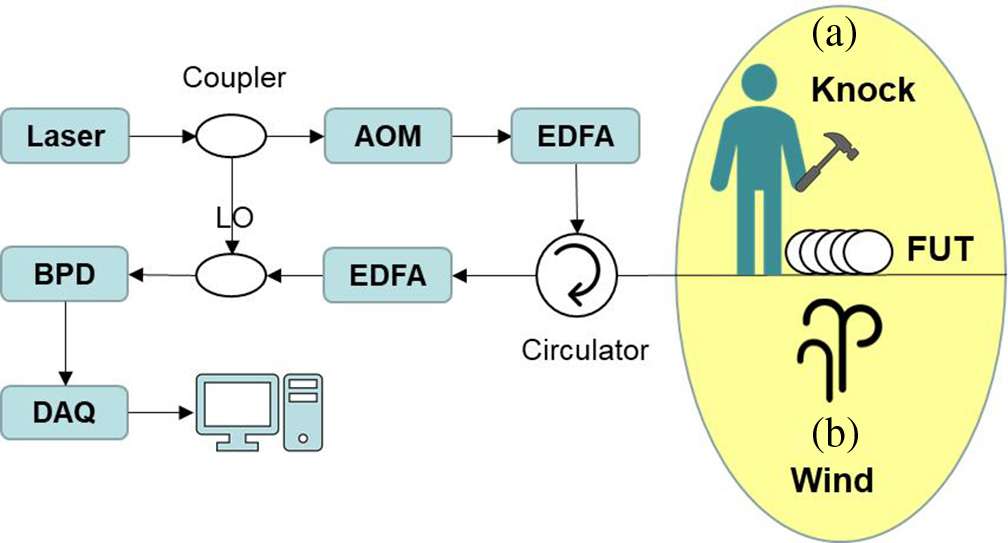
The setup of the involved φ-OTDR system is shown in Fig. 1. Figure 2(a) shows the developed prototype φ-OTDR instrument, and Fig. 2(b) shows the deployed fiber in experiment. An ultranarrow linewidth laser is used as the light source. The output light of the laser is divided into two beams by a 99:1 coupler. The 99% light serves as the probe light, and the 1% section is the local oscillator light. The probe light is modulated into pulsed light by an acoustic-optic modulator (AOM), amplified by an erbium-doped fiber amplifier (EDFA). Then the probe pulse light is injected into the sensing fiber through the circulator. Then, the Rayleigh backscattered signal and local oscillator light are mixed in a 50:50 coupler and converted into an electrical signal by a balanced photodetector (BPD). The electrical signal is received by the data acquisition card (DAQ). Corresponding digital signal processing (DSP) is performed on the collected digital signals to obtain information, including the location of the disturbance and the frequency of the disturbance signal, which is shown in Fig. 2. The probe pulse width is set as 100 ns, and the repetition period is 2 µs. The frequency shift of the AOM is 80 MHz, and the DAQ sampling rate is 200 MS/s. The spatial resolution of the φ-OTDR system is 10 m.

When the vibration signal is applied to the fiber, the phase of the Rayleigh backscattering (RBS) signal in the disturbed region is modulated accordingly. The RBS signal after the disturbance can be expressed as Icom(t)=EsELOcos(Δφ)+jEsELOsin(Δφ),(1)where EsELOis the intensity of the RBS signal, and Δφ is the phase of the RBS signal. Icom(t) is converted into a trace matrix. The received RBS signal can be converted to the data matrix, as shown in Fig. 3. The first dimension of the matrix is named “fast time,” which represents the distance along the fiber. The second dimension of the trace matrix, which is termed “slow time,” is the time axis of the RBS signal at each location of the fiber^[25]. The angle function is used to extract the phase of the trace matrix signal, as shown in the following: Δφ=angle(EsELOejΔφ).(2)

Then STFT is performed on the obtained disturbed signal to obtain the time-frequency diagram^[18]. The basic calculation is S(z,f)=∫−∞∞i(z)g(z−τ)exp(−j2πfz)dz,(3)where i(z) is the disturbance signal; g(z−τ) is the time window centered on τ; and exp(−j2πfz) is a modulation operator that converts the signal from the time domain to the frequency domain.

After selecting the STFT window function, the resolution is fixed when the window length function is determined. Since the time resolution is inversely proportional to the frequency resolution, they cannot be optimized simultaneously. Therefore, choosing the appropriate window function type and reasonable window length is vital. Here we use the Hanning window function to intercept the signal to guarantee fine-frequency resolution and less spectrum leakage. Its expression can be written as w(n)=12{1−cos[2π(n−1)N]},0≤n≤N−1,(4)where N is the length of the window. To obtain frequency resolution and facilitate calculation, the window length is set to 8192.

The data set greatly influences the recognition performance, and a reasonable data set structure is crucial for pattern recognition. Common vibration signals include mechanical activity, walking, wind blowing, rain, knocking, shaking, etc. In this paper, three typical event types, i.e., background noise, knocking, and wind blowing, are selected. The knock signal is obtained by striking with a hammer. A fan generates the wind blowing signal to simulate the natural wind blowing in the virtual environment. Background noise is obtained when the ambient environment is relatively quiet without any vibration event. The composition of the data set is shown in Table 1. The time-domain waveforms of different vibration events are presented in Fig. 4.

We have selected a range of 10 m in the spatial neighborhood of the vibration signal. Each temporal-spatial image represents a spatial length of 10 m and a temporal length of 1 s, shown in Figs. 5(a)–5(c), where the unit on the color bars is the radian (the unit of phase). The vertical and horizontal direction of the temporal-spatial image represents position and time, respectively. The time duration of time-frequency images is 1 s, which is shown in Figs. 5(d)–5(f). For the time-frequency image, the horizontal axis presents time too, whereas the vertical axis presents frequency. The unit of the color bars in Figs. 5(d)–5(f) is the decibel, where 0 dB refers to the maximum value of the whole spectrum along the position.

Deep-learning methods such as CNN can automatically learn the features of data sets. ResNet50 has a deep network level and few parameters, achieving good results in image data sets in other fields. Consequently, it is applied to φ-OTDR event classification. ResNet50 increases the network depth by stacking the remaining blocks to solve the network degradation problem and the vanishing gradient problem^[26–28]. Here we adopt ResNet50 network as the recognition classifier, as shown in Fig. 6. ResNet50 contains 50 conv2d operations, which are divided into five stages. The first convolution layer has 64 kernels. The size and maximum pooled stride of each kernel are 7×7 and 2, respectively. The last four stages have 9, 12, 18, and 9 convolution layers, also known as residual blocks, as shown in Fig. 7. x is the input to the residual block. F(x) is the output after linear change and activation. The figure shows that in the residual network, F(x) adds the input value x of this layer before activation after the linear change of the second layer, and then carries out the output after activation. X is added before the second layer output value is activated. This path is called a shortcut connection. The residual block is used to deepen the network. With the increase of the network, the global feature vector of the feature image is extracted (2048, 7, 7). The average pooling layer converts it into an eigenvector. After passing through the dropout layer, the 2048-dimensional feature vector is connected to the full connection layer. Finally, the classifier calculates the feature vector and outputs the category probability. For training, the model performs L2 regularization optimization on epochs. In addition, we trained the model using feature images to verify the effect of time and space on classification accuracy. The categorical cross-entropy loss uses the Adam optimizer and the ReLU activation function to speed up the computation. The model input is a 1×3×224×224 feature vector, and then the data are processed through two-dimensional convolution, max pooling, and fully connected layers.

Here, the ResNet50 classifier is used to train and validate the temporal-spatial and time-frequency images, respectively, and the cross-validation method is used to evaluate the classification results. The learning rate is set as 0.003. In deep learning, the principle of small-batch data processing is generally adopted. The batch size is 25, and the training epoch is 100. We collected 1200 sets of three signals: knock around the fiber with a hammer, the wind blowing optical fiber, and background noise. The ratio of the training set and validation set is 7:3. The loss and accuracy are obtained with each iteration, and the hyperparameters are changed to optimize the next training. Each network is tested in the test phase every 100 iterations. The resultant training loss and validation accuracy curves are shown in Fig. 8.

During the training on time-frequency images, the training loss, representing the network error, decreases slowly after 50 epochs until it hovers around 0.03, and the best test accuracy is 98%. In contrast, the test accuracy of the temporal-spatial image is 99%, and the training loss reaches 0.01 after 30 epochs. The results show that the classification performance based on the temporal-spatial images is better. The classification results are shown in Table 2, which shows that classification accuracy based on the temporal-spatial images achieves 99.49%, whereas the classification accuracy based on time-frequency images is 98.23%. The accuracy of temporal-spatial images is 1.33% higher than that of the time-frequency images. From the average training time per step, the temporal-spatial map as input is improved by 3 s compared to the time-frequency map as input. However, from Table 3 it is clear that the recall and f1-score of the input time-frequency image reach 100%, indicating that the model has a better recognition effect on the time-frequency characteristics of continuous signals. The confusion matrices are shown in Fig. 9. The knocking signal is most easily confused compared with the other two types of signals, primarily based on time-frequency characteristics. A possible explanation is that the knock signal is a single point tapping signal that is transient in the time domain. There is a time difference between the two disturbance signals. The signal feature image will contain the interference information of the external environment.

The experimental results show that the classification effect based on the temporal-spatial image is better than that of the time-frequency image. In preprocessing the two signals, the extraction of the temporal-spatial feature does not require precise positioning in advance. Taking the distance within the range of 20 m around the perturbation position, we have converted the signal of this distance into a temporal-spatial image. The temporal and spatial correlation of the signal is preserved, and the intensity information is extracted from the image. The temporal-spatial features are directly extracted by the CNN model, which avoids manual processing during the classification, thereby reducing the workload and retaining the features of the original signal. However, the time-frequency feature extracted by STFT must locate the disturbance signal. The time-frequency features extracted by STFT need to locate the disturbance signals and extract the signal features. In practical applications, most of the collected signals are discontinuous signals. Due to external disturbance, it is difficult to accurately extract target disturbance information, and there may be some information loss. Therefore, the extraction of time-frequency feature information is greatly affected by the environment, resulting in a slightly worse classification effect.

This paper compares and analyzes the disturbance events classification methods in φ-OTDR using different features of CNN, namely, temporal-spatial features and time-frequency features. Through the experiments on a 3600-sample data set, temporal-spatial and time-frequency images are directly used as the input of the ResNet50. The temporal-spatial images based classification accuracy achieves 99.49%, and the classification accuracy of time-frequency images is 98.23%. Training accuracy, valid accuracy, average training time, loss curve, and confusion matrix are used as evaluation criteria. Due to the disturbance of the external environment, the space range of time-frequency feature extraction is short, and there is interference in feature extraction for the transient signals, such as knocking. The temporal-spatial image of the signal has good space–time correlation, and the extracted features contain complete information. Therefore, the classification effect of temporal-spatial images is better than that of time-frequency images. The recognition results of the two feature images provide meaningful reference for the further study of pattern recognition in φ-OTDR.

References

[1] H. Meng, S. Wang, C. Gao, F. Liu. Research on recognition method of railway perimeter intrusions based on Φ-OTDR optical fiber sensing technology. IEEE Sens. J., 21, 9852(2021).
[2] H. Wu, X. Liu, Y. Xiao, Y. Rao. A dynamic time sequence recognition and knowledge mining method based on the hidden Markov models (HMMs) for pipeline safety monitoring with Φ-OTDR. J. Light. Technol., 37, 4991(2019).
[3] H. Wu, J. Chen, X. Liu, Y. Xiao, M. Wang, Y. Zheng, Y. Rao. One-dimensional CNN-based intelligent recognition of vibrations in pipeline monitoring with DAS. J. Light. Technol., 37, 4359(2019).
[4] Y. Lu, T. Zhu, L. Chen, X. Bao. Distributed vibration sensor based on coherent detection of phase-OTDR. J. Light. Technol., 28, 3243(2010).
[5] Z. Wang, Z. Pan, Q. Ye, B. Lu, Z. Fang, H. Cai, R. Qu. Novel distributed passive vehicle tracking technology using phase sensitive optical time domain reflectometer. Chin. Opt. Lett., 13, 100603(2015).
[6] Y. Zhang, T. Zhou, Z. Ding, Y. Lu, X. Zhang, F. Wang, N. Zou. Classification of interference-fading tolerant Φ-OTDR signal using optimal peak-seeking and machine learning [Invited]. Chin. Opt. Lett., 19, 030601(2021).
[7] H. Jia, S. Lou, S. Liang, X. Sheng. Event identification by F-ELM model for ϕ-OTDR fiber-optic distributed disturbance sensor. IEEE Sens. J., 20, 1297(2020).
[8] H. Wu, B. Zhou, K. Zhu, C. Shang, H.-Y. Tam, C. Lu. Pattern recognition in distributed fiber-optic acoustic sensor using intensity and phase stacked convolutional neural network with data augmentation. Opt. Express, 29, 3269(2021).
[9] M. Aktas, T. Akgun, M. U. Demircin, D. Buyukaydin. Deep learning based multi-threat classification for phase-OTDR fiber optic distributed acoustic sensing applications. Proc. SPIE, 10208, 102080G(2017).
[10] Z. Wang, Z. Pan, Q. Ye, B. Lu, H. Cai, R. Qu, Z. Fang, H. Zhao. Vehicle tracking by φ-OTDR used in safety monitored areas. Opto-Electronics and Communications Conference (OECC), 1(2015).
[11] H. Liu, F. Pang, L. Lv, X. Mei, Y. Song, J. Chen, T. Wang. True phase measurement of distributed vibration sensors based on heterodyne φ-OTDR. IEEE Photon. J., 10, 7101309(2018).
[12] H. F. Taylor, C. E. Lee. Apparatus and method for fiber optic intrusion sensing. U.S. patent.
[13] X. Chen, C. Xu. Disturbance pattern recognition based on an ALSTM in a long-distance φ-OTDR sensing system. Microw. Opt. Technol. Lett., 62, 168(2019).
[14] M. Zhang, Y. Li, J. Chen, Y. Song, J. Zhang, M. Wang. Event detection method comparison for distributed acoustic sensors using φ-OTDR. Opt. Fiber Technol., 52, 101980(2019).
[15] H. Wu, M. Yang, S. Yang, H. Lu, C. Wang, Y. Rao. A novel DAS signal recognition method based on spatiotemporal information extraction with 1DCNNs-BiLSTM network. IEEE Access, 8, 119448(2020).
[16] D. He, C. Liu, Z. Jin, R. Ma, Y. Chen, S. Shan. Fault diagnosis of flywheel bearing based on parameter optimization variational mode decomposition energy entropy and deep learning. Energy, 239, 122108(2022).
[17] M. Aktas, T. Akgun, M. U. Demircin, D. Buyukaydin. Deep learning based threat classification in distributed acoustic sensing systems. 25th Signal Processing and Communications Applications Conference (SIU), 1(2017).
[18] C. Xu, J. Guan, M. Bao, J. Lu, W. Ye. Pattern recognition based on time-frequency analysis and convolutional neural networks for vibrational events in φ-OTDR. Opt. Eng., 57, 016103(2018).
[19] Y. Shi, Y. Li, Y. Zhang, Z. Zhuang, T. Jiang. An easy access method for event recognition of φ-OTDR sensing system based on transfer learning. J. Light. Technol., 39, 4548(2021).
[20] H. Wu, S. Xiao, X. Li, Z. Wang, J. Xu, Y. Rao. Separation and determination of the disturbing signals in phase-sensitive optical time domain reflectometry (Φ-OTDR). J. Light. Technol., 33, 3156(2015).
[21] Y. Wang, P. Wang, K. Ding, H. Li, J. Zhang, X. Liu, Q. Bai, D. Wang, B. Jin. Pattern recognition using relevant vector machine in optical fiber vibration sensing system. IEEE Access, 7, 5886(2019).
[22] Z. Wang, S. Lou, S. Liang, X. Sheng. Multi-class disturbance events recognition based on EMD and XGBoost in φ-OTDR. IEEE Access, 8, 63551(2020).
[23] Z. Wang, L. Li, H. Zheng, J. Liang, X. Wang, B. Lu, Q. Ye, H. Cai, R. Qu. Smart distributed acoustics/vibration sensing with dual path network. 26th International Conference on Optical Fiber Sensors, WF105(2018).
[24] Y. Shi, S. Dai, T. Jiang, Z. Fan. A recognition method for multi-radial-distance event of φ-OTDR system based on CNN. IEEE Access, 9, 143473(2021).
[25] Z. Wang, L. Zhang, S. Wang, N. Xue, F. Peng, M. Fan, W. Sun, X. Qian, J. Rao, Y. Rao. Coherent Φ-OTDR based on I/Q demodulation and homodyne detection. Opt. Express, 24, 853(2016).
[26] P. Khojasteh, L. A. Passos, T. Carvalho, E. Rezende, B. Aliahmad, J. P. Papa, D. K. Kumar. Exudate detection in fundus images using deeply-learnable features. Comput. Biol. Med., 104, 62(2019).
[27] A. S. B. Reddy, D. S. Juliet. Transfer learning with ResNet-50 for malaria cell-image classification. International Conference on Communication and Signal Processing (ICCSP), 945(2019).
[28] T. Zhou, X. Zhang, B. Kang, M. Chen. Multimodal fusion recognition for digital twin. Digit. Commun. Netw.(2022).
Set citation alerts for the article
Please enter your email address
© Copyright 2018-2021 | Chinese Laser Press. All Rights Reserved 沪ICP备15018463号-20