• Photonics Research
  • Vol. 4, Issue 2, 0049 (2016)
S. C. V. Latas
Author Affiliations
  • I3N—Institute of Nanostructures, Nanomodelling and Nanofabrication, Department of Physics, University of Aveiro, 3810-193 Aveiro, Portugal
  • show less
    DOI: 10.1364/prj.4.000049 Cite this Article Set citation alerts
    S. C. V. Latas. High-energy plain and composite pulses in a laser modeled by the complex Swift–Hohenberg equation[J]. Photonics Research, 2016, 4(2): 0049 Copy Citation Text show less
    Region of existence of dissipative solitons (darker area), in the plane (ϵ, D), for the following parameter values: β=−0.3, δ=−0.5, μ=−0.001, ν=0, and γ=0.05. Dissipative pulses do not exist beyond the lower and upper boundaries. Nevertheless, their region of existence extends beyond the left and right boundaries, for values of |D|>2. The marks (circles, squares, and triangles) correspond to examples of pulses presented in the following figures.
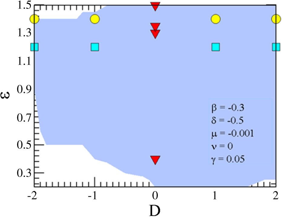
    Fig. 1. Region of existence of dissipative solitons (darker area), in the plane (ϵ, D), for the following parameter values: β=0.3, δ=0.5, μ=0.001, ν=0, and γ=0.05. Dissipative pulses do not exist beyond the lower and upper boundaries. Nevertheless, their region of existence extends beyond the left and right boundaries, for values of |D|>2. The marks (circles, squares, and triangles) correspond to examples of pulses presented in the following figures.
    (a) Amplitude and (b) spectral pulse profiles for four values of ϵ, namely, ϵ=0.4 (thick dashed curves), ϵ=1.3 (solid curves), ϵ=1.35 (dashed–dotted curves), and ϵ=1.5 (dashed curves). The curves correspond to the triangles along the vertical line D=0 in Fig. 1. (The other parameter values are β=−0.3, δ=−0.5, μ=−0.001, ν=0, and γ=0.05.)
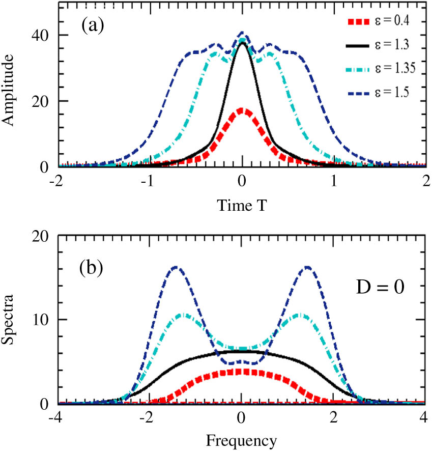
    Fig. 2. (a) Amplitude and (b) spectral pulse profiles for four values of ϵ, namely, ϵ=0.4 (thick dashed curves), ϵ=1.3 (solid curves), ϵ=1.35 (dashed–dotted curves), and ϵ=1.5 (dashed curves). The curves correspond to the triangles along the vertical line D=0 in Fig. 1. (The other parameter values are β=0.3, δ=0.5, μ=0.001, ν=0, and γ=0.05.)
    Energy Q of dissipative pulses versus dispersion parameter, D, for three different values of ϵ, associated with PPs, NCPs, and WCPs.
    Fig. 3. Energy Q of dissipative pulses versus dispersion parameter, D, for three different values of ϵ, associated with PPs, NCPs, and WCPs.
    Pulses’ (a) amplitude, (b) chirp, and (c) spectra for four different values of D. The pulse curves correspond to the squares along the horizontal line ϵ=1.2 in Fig. 1. (The other parameter values are β=−0.3, δ=−0.5, μ=−0.001, ν=0, and γ=0.05.)
    Fig. 4. Pulses’ (a) amplitude, (b) chirp, and (c) spectra for four different values of D. The pulse curves correspond to the squares along the horizontal line ϵ=1.2 in Fig. 1. (The other parameter values are β=0.3, δ=0.5, μ=0.001, ν=0, and γ=0.05.)
    Pulse (a) amplitudes, (b) chirp, and (c) spectra for the same four different values of D as in Fig. 4. The pulses represented are WCPs for D<0 and NCPs for D>0. Similar profiles of WCPs and NCPs were obtained in both dispersion regimes. The pulse curves correspond to the circles along the horizontal line ϵ=1.4 in Fig. 1. (The other parameter values are β=−0.3, δ=−0.5, μ=−0.001, ν=0, and γ=0.05.)
    Fig. 5. Pulse (a) amplitudes, (b) chirp, and (c) spectra for the same four different values of D as in Fig. 4. The pulses represented are WCPs for D<0 and NCPs for D>0. Similar profiles of WCPs and NCPs were obtained in both dispersion regimes. The pulse curves correspond to the circles along the horizontal line ϵ=1.4 in Fig. 1. (The other parameter values are β=0.3, δ=0.5, μ=0.001, ν=0, and γ=0.05.)
    Pulse (a) evolution, (b) amplitude, and (c) spectrum profiles of a plain pulse solution. A small change in some parameter values can produce a significant growth of the pulse amplitude. [The parameter values are D=0, β=−0.3, δ=−0.5, ϵ=0.35, μ=0, ν=−0.000025, and γ=0.05, as shown in (b).]
    Fig. 6. Pulse (a) evolution, (b) amplitude, and (c) spectrum profiles of a plain pulse solution. A small change in some parameter values can produce a significant growth of the pulse amplitude. [The parameter values are D=0, β=0.3, δ=0.5, ϵ=0.35, μ=0, ν=0.000025, and γ=0.05, as shown in (b).]
    S. C. V. Latas. High-energy plain and composite pulses in a laser modeled by the complex Swift–Hohenberg equation[J]. Photonics Research, 2016, 4(2): 0049
    Download Citation