S. C. V. Latas
Abstract
In this work, new plain and composite high-energy solitons of the cubic–quintic Swift–Hohenberg equation were numerically found. Starting from a composite pulse found by Soto-Crespo and Akhmediev and changing some parameter values allowed us to find these high energy pulses. We also found the region in the parameter space in which these solutions exist. Some pulse characteristics, namely, temporal and spectral profiles and chirp, are presented. The study of the pulse energy shows its independence of the dispersion parameter but its dependence on the nonlinear gain. An extreme amplitude pulse has also been found.1. INTRODUCTION
Laser systems with passive mode locking can be described by the cubic–quintic complex Ginzburg–Landau (CGLE) and Swift–Hohenberg (CSHE) equations [1]. Both equations have a wide diversity of analytical and numerical solutions, as can be seen for example in [1–6], and references therein. Among other characteristics, both models have in common two particular numerical solutions: the plain and the composite solitons [6–9].
Recently, ultrashort high-energy pulses and extreme amplitude spikes, solutions of the CGLE, have been found [10,11].
Such diversity and complexity of solutions is due, in part, to the fact that the CGLE has several free parameters. A small change of one of these parameters can have a huge impact on the nature of the solution [11].
Sign up for Photonics Research TOC. Get the latest issue of Photonics Research delivered right to you!Sign up now
Some technological applications of high-energy pulses are, for example, dissipative soliton fiber lasers in the normal dispersion regime or with parameter management [12–14].
One of the restrictions of the CGLE model concerns spectral filtering, which is limited to a second-order term, characterized by a single maximum spectral response. In general, in experiments the gain spectrum is large and might have several maxima. For more realistic modeling it is necessary to add higher-order spectral filtering terms. The addition of a fourth-order spectral filtering term into the cubic–quintic CGLE transforms it into the CSHE [1,6]. The role of this higher-order term in spectral filtering has been studied in [6]. In particular, narrow composite pulse (NCP) and wider composite pulse (WCP) were numerically found.
In this work new plain and composite high-energy solitons of the CSHE, and their region of existence in the plane (, ), have been numerically found. Some pulse characteristics are presented. Additionally, a plain pulse with extreme amplitude peak was also found.
2. THEORY
The CSHE can be written in the following form [1,6]: where is the propagation distance or the cavity round-trip number, is the retarded time in a frame of reference moving with the group velocity, and is the normalized complex envelope of the optical field. On the left-hand side, represents the cavity dispersion, with in the anomalous regime and in the normal regime, and corresponds, if negative, to the saturation of the nonlinear refractive index. On the right-hand side, represents the difference between linear gain and loss; and account for spectral filtering and higher order spectral filtering, respectively. The terms with and , represent the nonlinear gain and the saturation of the nonlinear gain, respectively.
The CSHE given by Eq. (1) has been numerically solved, with a split-step Fourier symmetric method, with a time step and a distance step , described for example in [15]. Absorbing boundary conditions were used, as presented in [16]. In order to guarantee the convergence to a single pulse, an initial condition of the form has been considered. For initial conditions with a larger width multiple pulses can be formed.
3. RESULTS
At this stage we refer that the starting point for this work was the composite pulse (CP), discovered in [6] for the following set of parameter values: , , , , , and . We might ask, what is the impact of a small change of the saturation of the nonlinear gain, , on the nature of the solution? The pulse amplitude is gradually reduced as becomes slightly more negative. On the other hand, as the pulse amplitude grows. If , blow-up occurs. Hence, in this case, the saturation of the nonlinear gain is the physical mechanism that prevents the growth of the pulse amplitude against blow-up, since .
The region of existence in the plane (, ) of the high-energy pulses that were found in this work is presented in Fig. 1, for the following parameter values: , , , , and . Note that these values are similar to the ones found in [6], except the value.
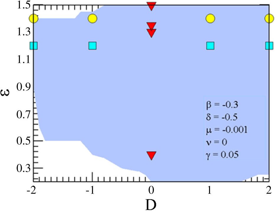
Figure 1.Region of existence of dissipative solitons (darker area), in the plane (, ), for the following parameter values: , , , , and . Dissipative pulses do not exist beyond the lower and upper boundaries. Nevertheless, their region of existence extends beyond the left and right boundaries, for values of . The marks (circles, squares, and triangles) correspond to examples of pulses presented in the following figures.
Moreover, the filter spectral response, , exhibits a double peak structure which was also the one presented in [6]. Dissipative pulses exist for both normal () and anomalous () dispersion regimes. This region extends beyond the left and right boundaries for . Beyond the lower and upper boundaries dissipative solitons do not exist. Below the lower boundary the pulses in general decay or coexist with moving strongly asymmetric pulses. Above the upper boundary the pulses expand ().
Typical pulse shapes and spectra are presented in Figs. 2–4. In Fig. 2 the pulses represented correspond to the triangles along the vertical line (the zero dispersion point) in Fig. 1. For each distinct value of similar profiles were found. From Fig. 2(a), as the cubic nonlinear gain, , increases, the pulses shapes change dramatically from plain pulses (PPs) to NCP and WCP. In general, for all values of in the region, NCP and WCP coexist for . It can be seen that the higher amplitude peak pulse () or peak intensity, 1600, occurs for a nonlinear gain value of . This amplitude is significantly higher if compared with the maximum value of the peak pulse () for , presented in [10]. In the spectral domain, with the increase of the pulses’ spectral amplitudes, , grow [Fig. 2(b)]. The spectra of PPs exhibit a single maximum, whereas the CPs exhibit a dual peak spectra. These results are in good agreement with the results obtained in [6–9] for PPs and CPs with lower energies in the context of the Ginzburg–Landau and Swift–Hohenberg equations, respectively. However, the pulses’ spectral widths are smaller than the ones presented in [10].

Figure 2.(a) Amplitude and (b) spectral pulse profiles for four values of , namely, (thick dashed curves), (solid curves), (dashed–dotted curves), and (dashed curves). The curves correspond to the triangles along the vertical line in Fig. 1. (The other parameter values are , , , , and .)
The pulse energies, , are 116, 448, 1179, and 2051 for , 1.3, 1.35, and 1.5, respectively.
The pulse energies versus are presented in Fig. 3 for three different values of nonlinear gain, . The pulse energies are similar or even higher than the ones presented in [10].
Figure 3.Energy of dissipative pulses versus dispersion parameter, , for three different values of , associated with PPs, NCPs, and WCPs.
Figure 4.Pulses’ (a) amplitude, (b) chirp, and (c) spectra for four different values of . The pulse curves correspond to the squares along the horizontal line in Fig. 1. (The other parameter values are , , , , and .)
Figure 5.Pulse (a) amplitudes, (b) chirp, and (c) spectra for the same four different values of as in Fig. 4. The pulses represented are WCPs for and NCPs for . Similar profiles of WCPs and NCPs were obtained in both dispersion regimes. The pulse curves correspond to the circles along the horizontal line in Fig. 1. (The other parameter values are , , , , and .)
The results in Fig. 3 show that the pulse energies are practically independent of the values of dispersion in both the normal and anomalous regimes, and increase as increases. For and only PPs are formed, and for NCPs and WCPs coexist with different values of energy. In general, for the higher considered values of , the energies of each kind of pulse slightly decrease with , whereas for the lower considered values the opposite occurs. This behavior contrasts with the unlimited growth of energy as decreases, for similar values of as the high-energy pulses presented in [10].
Figures 4 and 5 illustrate the two different kinds of high-energy pulses found, namely PPs and CPs.
The pulses represented in Fig. 4 correspond to the squares along the horizontal line in Fig. 1. In Fig. 4(a) the pulse amplitude profiles are presented for four different values of . All the four pulses shapes are pretty similar and consequently almost independent of . The major difference occurs at the pulse wings.
As increases, less energy is concentrated at the wings, while the peak amplitude remains almost the same.
Figure 4(b) shows that the pulses are chirped, with a linear chirp across the pulse central region. In the transition between the pulse central region and the pulse wings a small deep and a small crest occur at the leading and trailing edges, respectively. The presence of chirp makes it possible to carry out pulse compression and hence obtain high-energy, ultrashort pulses [14].
Figure 4(c) shows the pulses’ spectra profiles. As should be expected, the pulses’ spectra are very similar to each other. The spectrum of each pulse has a single maximum, and most of the energy is concentrated between the frequencies and 2. If we compare theses pulses with the ones obtained in the context of CGLE [10], for several values of , it can be seen that in the temporal domain the pulses exhibit higher amplitudes than the CGLE pulses, for a smaller value of the nonlinear gain parameter. Nevertheless, in the spectral domain their spectral widths are much smaller than the ones exhibited by the CGLE pulses.
Figure 5 presents the pulses that correspond to the circles along the horizontal line in Fig. 1.
In Fig. 5(a) the pulses’ amplitude profiles are presented for four different values of . Two different kind of pulses are formed, namely a NCP and a WCP. The represented pulses are WCPs for and NCPs for . Both kinds of pulses coexist for and for all considered values of in Fig. 1, with similar amplitude profiles. In general, if a NCP is generated from a , the coexisting WCP can be obtained from an initial condition whose width is slightly larger. And if a WCP is generated, a NCP can be obtained from an initial condition whose width is slightly smaller. As can be seen, the pulses’ peak amplitudes and profiles are almost the same for different values of .
In Fig. 5(b) the pulses’ chirps are represented in the temporal domain. Across the pulses’ central region the chirp is linear. Small deeps and crests appear in the transition from the pulses’ central region to the pulses’ edges, following the multipeak structure. In these cases the chirp is far for being linear across the whole pulse. However, some compression might be possible. A detailed discussion of high-energy chirped pulse compression is presented in [14].
Pulses spectral profiles are represented in Fig. 5(c). As should be expected, the NCP and WCP have dual peak spectra. The spectral width is similar for both cases. Nevertheless, the spectral peak structure is different, with the WCPs having higher peak amplitude than the NCPs. On the other hand, the deeps between the two peaks, as well as the peak separations, are larger for the WCPs than for NCPs.
The amplitude of the pulses may have a substantial increase if we change the parameter values as presented in Fig. 6, for the following parameter values: , , , , , , and .
Figure 6.Pulse (a) evolution, (b) amplitude, and (c) spectrum profiles of a plain pulse solution. A small change in some parameter values can produce a significant growth of the pulse amplitude. [The parameter values are , , , , , , and , as shown in (b).]
Figure 6 shows the pulse’s (a) amplitude evolution, (b) amplitude, and (c) spectrum profiles of an extreme amplitude plain pulse solution obtained from an initial condition of , with and . The characteristics of this pulse are similar to the PP presented in Fig. 4. As can be seen, the pulse peak amplitude is almost 326 for peak intensity 106207, with energy . To the best of our knowledge, this is one of the highest peak amplitudes found in the context of the CSHE and CGLE. In this case the physical mechanism that restricts the growth of the pulse amplitude against blow-up is the saturation of the nonlinear refractive index, , since . Based on our results we predict the existence of even higher extreme amplitude pulses, but further research will be necessary.
4. CONCLUSION
In conclusion, new plain and composite high-energy solitons of the cubic–quintic Swift–Hohenberg equation have been numerically found. These new solutions have high energy if compared with the traditional PPs and CPs known for this model. A region of existence of these pulses was also found in the plane (, ). The pulses exist in both normal and anomalous dispersion regimes. For a specific value of the cubic nonlinear gain, , the energy of each kind of pulse, namely PP, NCP, and WCP, is almost independent of . However, the pulses’ energies are high but finite. A change of the parameter values allows us to find an extreme amplitude plain pulse.
ACKNOWLEDGMENT
Acknowledgment. I thank M. Facão for useful discussions. I acknowledge FCT (Fundação para a Ciência e Tecnologia) for supporting this work through the Project UID/CTM/50025/2013.
References
[1] N. Akhmediev, A. Ankiewicz. Dissipative Solitons(2005).
[2] J. Lega, J. Moloney, A. Newell. Swift–Hohenberg equation for lasers. Phys. Rev. Lett., 73, 2978-2981(1994).
[3] H. Sakaguchi, H. Brand. Localized patterns for the quintic complex Swift–Hohenberg equation. Phys. D, 117, 95-105(1998).
[4] I. Aranson, L. Kramer. The world of the complex Ginzburg–Landau equation. Rev. Mod. Phys., 74, 99-143(2002).
[5] K. Maruno, A. Ankiewicz, N. Akhmediev. Exact soliton solutions of the one-dimensional complex Swift–Hohenberg equation. Phys. D, 176, 44-66(2003).
[6] J. Soto-Crespo, N. Akhmediev. Composite solitons and two-pulse generation in passively mode-locked lasers modeled by the complex quintic Swift–Hohenberg equation. Phys. Rev. E, 66, 066610(2002).
[7] H. Wang, L. Yanti. An efficient numerical method for the quintic complex Swift–Hohenberg equation. Numer. Math. Theor. Appl., 4, 237-254(2011).
[8] V. Afanajev, N. Akhmediev, J. Soto-Crespo. Three forms of localized solutions of the quintic complex Ginzburg–Landau equation. Phys. Rev. E, 53, 1931-1939(1996).
[9] N. Akhmediev, A. Rodrigues, G. Town. Interaction of dual frequency pulses in passively mode-locked lasers. Opt. Commun., 187, 419-426(2001).
[10] N. Akhmediev, J. Soto-Crespo, P. Grelu. Roadmap to ultra-short record high-energy pulses out of laser oscillators. Phys. Lett. A, 372, 3124-3128(2008).
[11] W. Chang, J. Soto-Crespo, P. Vouzas, N. Akhmediev. Extreme amplitude spikes in a laser model described by the complex Ginzburg–Landau equation. Opt. Lett., 40, 2949-2952(2015).
[12] Z. Liu, S. Zhang, F. Wise. Rogue waves in a normal dispersion fiber laser. Opt. Lett., 40, 1366-1369(2015).
[13] C. Lecaplain, P. Grelu, J. M. Soto-Crespo, N. Akhmediev. Dissipative rogue waves generated by chaotic pulse bunching in a mode-locked laser. Phys. Rev. Lett., 108, 233901(2012).
[14] W. Chang, A. Ankiewicz, J. Soto-Crespo, N. Akhmediev. Dissipative soliton resonances in laser models with parameter management. J. Opt. Soc. Am. B, 25, 1972-1977(2008).
[15] M. Ferreira. Nonlinear Effects in Optical Fibers(2011).
[16] F. If, P. Berg, P. L. Christiansen, O. Skovgaard. Split-step spectral method for nonlinear Schrodinger-equation with absorbing boundaries. J. Comp. Phys., 72, 501-503(1987).


