• Photonics Research
  • Vol. 7, Issue 3, 368 (2019)
Tian Zhang1, Jia Wang1, Qi Liu1, Jinzan Zhou1, Jian Dai1, Xu Han2, Yue Zhou1, and Kun Xu1、*
Author Affiliations
  • 1State Key Laboratory of Information Photonics and Optical Communications, Beijing University of Posts and Telecommunications, Beijing 100876, China
  • 2Huawei Technologies Co., Ltd., Shenzhen 518129, China
  • show less
    DOI: 10.1364/PRJ.7.000368 Cite this Article Set citation alerts
    Tian Zhang, Jia Wang, Qi Liu, Jinzan Zhou, Jian Dai, Xu Han, Yue Zhou, Kun Xu. Efficient spectrum prediction and inverse design for plasmonic waveguide systems based on artificial neural networks[J]. Photonics Research, 2019, 7(3): 368 Copy Citation Text show less
    Schematic diagrams of the (a) THRC system, (b) FORC system, and (c) FIRC system.
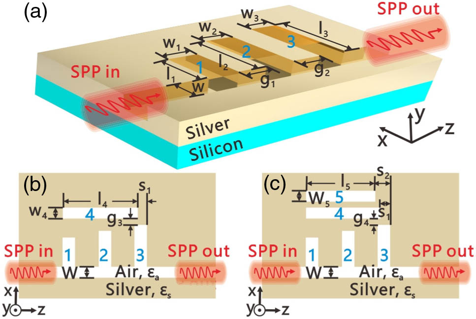
    Fig. 1. Schematic diagrams of the (a) THRC system, (b) FORC system, and (c) FIRC system.
    (a) Simulated transmission spectrum of the THRC system for Ag with loss (red solid line) and without loss (orange solid line), and theoretical transmission spectrum of the THRC system (blue dashed line); (b) group index and loss factor of the THRC system. The insets are simulated magnetic field distributions for the incident light at wavelengths of (A) 851 nm, (B) 893 nm, (C) 955 nm, (D) 1005 nm, and (E) 1048 nm.
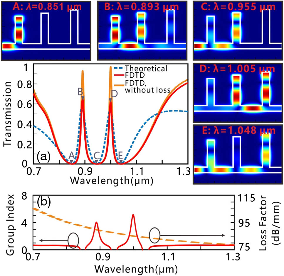
    Fig. 2. (a) Simulated transmission spectrum of the THRC system for Ag with loss (red solid line) and without loss (orange solid line), and theoretical transmission spectrum of the THRC system (blue dashed line); (b) group index and loss factor of the THRC system. The insets are simulated magnetic field distributions for the incident light at wavelengths of (A) 851 nm, (B) 893 nm, (C) 955 nm, (D) 1005 nm, and (E) 1048 nm.
    (a) Simulated transmission spectrum of the FORC system for g3=20 nm (red solid line) and 30 nm (orange solid line); theoretical transmission spectrum of the FORC system (blue circles); simulated transmission spectrum of the FORC system, which includes only cavities 1, 2, 4 (orange dashed line) and cavities 1, 2 (blue dashed line); (b) group index of the FORC system. The insets are calculated magnetic field distributions for the incident light at wavelengths of (A) 0.851 μm, (B) 0.893 μm, (C) 0.953 μm, (D) 1.01 μm, (E) 1.056 μm, (F) 1.168 μm, and (G) 1.18 μm.
    Fig. 3. (a) Simulated transmission spectrum of the FORC system for g3=20  nm (red solid line) and 30 nm (orange solid line); theoretical transmission spectrum of the FORC system (blue circles); simulated transmission spectrum of the FORC system, which includes only cavities 1, 2, 4 (orange dashed line) and cavities 1, 2 (blue dashed line); (b) group index of the FORC system. The insets are calculated magnetic field distributions for the incident light at wavelengths of (A) 0.851 μm, (B) 0.893 μm, (C) 0.953 μm, (D) 1.01 μm, (E) 1.056 μm, (F) 1.168 μm, and (G) 1.18 μm.
    (a) Simulated transmission spectrum of the FIRC system for g4=40 nm (red solid line) and 60 nm (orange solid line); theoretical transmission spectrum of the FIRC system (blue dashed line); (b) group index of the FIRC system. The insets are calculated magnetic field distributions for the incident light at wavelengths of (A) 851 nm, (B) 893 nm, (C) 954 nm, (D) 1010 nm, (E) 1056 nm, (F) 1151 nm, (G) 1160 nm, (H) 1178 nm, and (I) 1189 nm.
    Fig. 4. (a) Simulated transmission spectrum of the FIRC system for g4=40  nm (red solid line) and 60 nm (orange solid line); theoretical transmission spectrum of the FIRC system (blue dashed line); (b) group index of the FIRC system. The insets are calculated magnetic field distributions for the incident light at wavelengths of (A) 851 nm, (B) 893 nm, (C) 954 nm, (D) 1010 nm, (E) 1056 nm, (F) 1151 nm, (G) 1160 nm, (H) 1178 nm, and (I) 1189 nm.
    (a) Diagram of the ANNs applied in the spectrum prediction; (b) fitness for different generations in the spectrum prediction; (c) training losses for different iterations in the spectrum prediction; FDTD simulated transmission spectra and ANN-predicted transmission spectra for the (d) THRC, (e) FORC, and (f) FIRC systems; (g) fitness for different generations in the parameter fitting. The inset reveals the training losses for different iterations in the parameter fitting.
    Fig. 5. (a) Diagram of the ANNs applied in the spectrum prediction; (b) fitness for different generations in the spectrum prediction; (c) training losses for different iterations in the spectrum prediction; FDTD simulated transmission spectra and ANN-predicted transmission spectra for the (d) THRC, (e) FORC, and (f) FIRC systems; (g) fitness for different generations in the parameter fitting. The inset reveals the training losses for different iterations in the parameter fitting.
    (a) Diagram of the ANNs applied in the inverse design and performance optimization problems; comparison results between the real structure parameters and ANN-predicted structure parameters for the (b) THRC, (c) FORC, and (d) FIRC systems. The insets in (b)–(d) are the FDTD-simulated transmission spectra corresponding to the real structures (red solid line) and ANN-predicted structure parameters (blue dashed line); (e) transmittance optimization for the THRC system; (f) bandwidth optimization for the FORC system; (g) transmittance optimization for the FIRC system.
    Fig. 6. (a) Diagram of the ANNs applied in the inverse design and performance optimization problems; comparison results between the real structure parameters and ANN-predicted structure parameters for the (b) THRC, (c) FORC, and (d) FIRC systems. The insets in (b)–(d) are the FDTD-simulated transmission spectra corresponding to the real structures (red solid line) and ANN-predicted structure parameters (blue dashed line); (e) transmittance optimization for the THRC system; (f) bandwidth optimization for the FORC system; (g) transmittance optimization for the FIRC system.
    Prediction accuracies for different numbers of training instances in the (a) spectrum prediction and (b) inverse design.
    Fig. 7. Prediction accuracies for different numbers of training instances in the (a) spectrum prediction and (b) inverse design.
    (a) The dispersion of Ag described by using the Drude model (red and blue solid lines) and experimental data (red and blue diamond-shaped markers), respectively; (b) transmission of THRC system when εAg is described by the Drude model (cyan solid line) and is set as a constant equal to −22.217+0.26i (orange solid line), −49.187+0.758i (yellow solid line), and −85.667+1.665i (purple solid line), corresponding to the εAg obtained by the Drude model at λ=0.7, 1, and 1.3 μm, respectively; (c) theoretically (triangle and inverted triangle markers) and numerically (blue solid and dashed lines) obtained nMDM of SPP mode supported by the MDM waveguide in the 2D case, and the numerically obtained nMDM in the 3D case at tcavity=300 nm (cyan solid and dashed lines), tcavity=500 nm (red solid and dashed lines), tcavity=700 nm (purple solid and dashed lines), and tcavity=900 nm (orange solid and dashed lines), respectively. The inset is the schematic of the 3D MDM cavity.
    Fig. 8. (a) The dispersion of Ag described by using the Drude model (red and blue solid lines) and experimental data (red and blue diamond-shaped markers), respectively; (b) transmission of THRC system when εAg is described by the Drude model (cyan solid line) and is set as a constant equal to 22.217+0.26i (orange solid line), 49.187+0.758i (yellow solid line), and 85.667+1.665i (purple solid line), corresponding to the εAg obtained by the Drude model at λ=0.7, 1, and 1.3 μm, respectively; (c) theoretically (triangle and inverted triangle markers) and numerically (blue solid and dashed lines) obtained nMDM of SPP mode supported by the MDM waveguide in the 2D case, and the numerically obtained nMDM in the 3D case at tcavity=300  nm (cyan solid and dashed lines), tcavity=500  nm (red solid and dashed lines), tcavity=700  nm (purple solid and dashed lines), and tcavity=900  nm (orange solid and dashed lines), respectively. The inset is the schematic of the 3D MDM cavity.
    Schematic diagram of the THRC system.
    Fig. 9. Schematic diagram of the THRC system.
    Schematic of the FORC system.
    Fig. 10. Schematic of the FORC system.
    Schematic of the FIRC system.
    Fig. 11. Schematic of the FIRC system.
    (a) Fitness of GA (blue) and PSO (black) for different generations in the inverse design; (b) comparison results between the ANN-predicted parameters, GA-optimized, and PSO-optimized structure parameters; (c) FDTD-simulated transmission spectra calculated for the ANN-predicted, GA-optimized, and PSO-optimized structure parameters.
    Fig. 12. (a) Fitness of GA (blue) and PSO (black) for different generations in the inverse design; (b) comparison results between the ANN-predicted parameters, GA-optimized, and PSO-optimized structure parameters; (c) FDTD-simulated transmission spectra calculated for the ANN-predicted, GA-optimized, and PSO-optimized structure parameters.
    Tian Zhang, Jia Wang, Qi Liu, Jinzan Zhou, Jian Dai, Xu Han, Yue Zhou, Kun Xu. Efficient spectrum prediction and inverse design for plasmonic waveguide systems based on artificial neural networks[J]. Photonics Research, 2019, 7(3): 368
    Download Citation