Abstract
In this paper, we propose a novel approach to achieve spectrum prediction, parameter fitting, inverse design, and performance optimization for the plasmonic waveguide-coupled with cavities structure (PWCCS) based on artificial neural networks (ANNs). The Fano resonance and plasmon-induced transparency effect originated from the PWCCS have been selected as illustrations to verify the effectiveness of ANNs. We use the genetic algorithm to design the network architecture and select the hyperparameters for ANNs. Once ANNs are trained by using a small sampling of the data generated by the Monte Carlo method, the transmission spectra predicted by the ANNs are quite approximate to the simulated results. The physical mechanisms behind the phenomena are discussed theoretically, and the uncertain parameters in the theoretical models are fitted by utilizing the trained ANNs. More importantly, our results demonstrate that this model-driven method not only realizes the inverse design of the PWCCS with high precision but also optimizes some critical performance metrics for the transmission spectrum. Compared with previous works, we construct a novel model-driven analysis method for the PWCCS that is expected to have significant applications in the device design, performance optimization, variability analysis, defect detection, theoretical modeling, optical interconnects, and so on.1. INTRODUCTION
Owing to the unique properties of near-field enhancement effect and breaking the diffraction limit, the emergence of surface plasmon polaritons (SPPs) has attracted a great deal of research attention [1]. Until now, diversified plasmonic structures have been proposed to excite and transmit the SPPs, such as metamaterial [2,3], dielectric gratings and metallic gratings [4,5], metal-dielectric-metal (MDM) waveguides [6–9], graphene-based waveguides [10,11], and hybrid waveguides [12–14]. In these structures, the plasmonic waveguide coupled with cavities structure (PWCCS), which can be easily integrated into plasmonic circuits, has attracted widespread attention because it is at subwavelength scale, supports a relatively long propagation length for SPPs, and demands relatively simple fabrication by using electron beam lithography and focused ion beam etching [14–16]. As for the simple PWCCSs, the physical mechanisms behind the phenomena are analyzed by utilizing some theoretical models and classical methods such as coupled-mode theory (CMT) and the transfer-matrix method (TMM) [6–9,17]. Then theoretical models are constructed to predict the transmission spectrum, determine structure parameters, and optimize some critical metrics (transmittance and bandwidth) [6–9]. However, for relatively complex PWCCSs with a complicated waveguide and cavity structure, the physical mechanism is hardly understood, and thus theoretical models are difficult to construct [18,19]. And the absence of an empirical relationship between the structure parameters and electromagnetic responses often enforces utilization of a time-consuming brute force search or evolutionary algorithms to determine the shape, dimensions, and variability of the device [20]. Obviously, an effective intelligence algorithm that obtains reliable spectrum prediction, inverse design, and performance optimization should be addressed in the design and analysis of photonic devices.
For the complex PWCCSs, computing the electromagnetic responses for all structure parameters via numerical simulation methods usually requires tremendous computation time. If the electromagnetic responses for all structure parameters can be predicted by using a small sampling of simulation results, the efficiency of design and analysis for complex PWCCSs will be improved. However, a simple and quick solution to predict and evaluate the spectrum responses for all structure parameters based on the partial simulation results is still lacking. In addition, although inverse design and performance optimization have been used to assist the design of mode multiplexers [21], wavelength multiplexers [22], polarization beam splitters [23], polarization rotators [24], power splitters [25], and so on, few studies have been focused on PWCCSs. Generally speaking, inverse design and performance optimization problems are solved by using several optimization algorithms, including gradient-based methods and gradient-free methods. For the gradient-based methods, the topology optimization solved by the adjoint method has been mostly applied in designing linear optical devices [21,22,26]. Recently, Hughes et al. have extended the traditional adjoint method to model nonlinear devices in the frequency domain [27]. For the gradient-free methods, evolution algorithms (genetic [24,28–30] and particle swarm [25]) and search algorithms (nonlinear search method [23]) are representative methods to design and optimize photonic devices. Among these optimization algorithms, the genetic algorithm (GA) is widely used because of its effectiveness, simplicity, and intuitiveness, even though it requires a lot of time to evolve, cross over, and mutate [28]. For example, directional optical cloaking and a gold nanostructure-based SPP sensor have been inversely designed by using the (micro) GA integrated with the finite-difference time-domain (FDTD) method [29,30]. Notably, these optimization algorithms usually optimize for some specific metrics, and they rarely directly achieve the most suitable structure parameters for a complete transmission spectrum in a wide wavelength range. In recent years, artificial neural networks (ANNs) have been applied in approximating many physics phenomena with high degrees of precision [31–40]. For example, the quantum many-body problem could be solved by utilizing ANNs [31]. Shen et al. pointed out that the trained ANNs could be used to simulate the light scattering of multilayer nanoparticles with different thicknesses [32]. And the trained ANNs could solve the spectrum prediction and inverse design problems more quickly than the numerical simulation method [32,33]. In order to avoid the data inconsistency problem in the inverse design for photonic devices, a tandem network structure composed of a forward-modeling unit and an inverse-design unit was proposed [34]. And ANN-based numerical methods have been proposed to design and optimize complex photonics devices, for example, power splitters [35], metagratings [20], and plasmonic devices [36–38]. Other machine-learning algorithms, such as reinforcement learning, the attractor selection algorithm, and the perceptron algorithm, were used to design subwavelength optical coupling devices and asymmetric light transmitters [39,40]. More interestingly, Liu et al. adopted a generative adversarial network that includes a generator and a critic to generate the essentially arbitrary metasurface patterns that yield a defined or optimized transmission spectrum [41]. It should be noted that the design of neural network architectures and the selection of hyperparameters for ANNs require a lot of expert knowledge [42]. Lately, GA [43], Bayesian optimization [44,45], and reinforcement learning [45] were tried for the automated design of ANNs. However, few studies in the above-mentioned works introduce the design process of the network architectures for ANNs, which is critical for prediction accuracy and algorithmic convergence.
In this paper, we propose a novel method using ANNs to achieve spectrum prediction, inverse design, and performance optimization for PWCCSs. To verify the effectiveness of ANNs, the Fano resonance (FR), especially for the plasmon-induced transparency (PIT) effect, originating from mode coupling in PWCCSs is taken into consideration. We use the GA to design the network architectures and select the suitable hyperparameters for ANNs. It is important to note that the transmission spectra predicted by ANNs are approximate to the FDTD simulated results with high precision. In addition, the physical mechanisms behind the FR and PIT effects are discussed based on the CMT and TMM, and the uncertain parameters in the theoretical models are fitted by using the trained ANNs effectively. Moreover, the ANNs have been successfully employed in solving the inverse design and performance optimization problems for PWCCSs.
Sign up for Photonics Research TOC. Get the latest issue of Photonics Research delivered right to you!Sign up now
2. DEVICE DESIGN AND SIMULATION RESULTS
It has been demonstrated that the FR and PIT effect can be found in the transmission spectrum of PWCCSs due to the mode coupling between the wideband bright modes and narrowband dark modes [6–9]. The PIT effect is often regarded as a special case of the FR whose spectrum line shape around the transmission peak is asymmetric [2]. Two different coupling methods are used to explain the FR and PIT effect in PWCCSs: one is based on the direct near-field coupling between bright modes and dark modes [8,46,47]; the other is based on the indirect destructive interference through waveguide shift coupling [6,7,9]. Correspondingly, the physical mechanisms of the FR and PIT effect can be explained by the destructive interference between two pathways in a three-level atomic system, including the ground, excited, and metastable states, or, equivalently, the doublet of dressed states [46]. In this paper, we construct three different PWCCSs that include different numbers of cavities as illustrations to verify the effectiveness of ANNs. Figure 1(a) exhibits the simplest three-resonators-coupled (THRC) system, which consists of an MDM waveguide and three side-coupled comb cavities. Compared with the THRC system [Fig. 1(a)], another one and two rectangular cavities are added in the up side of cavities 1, 2, and 3 to construct a four-resonators-coupled (FORC) system [Fig. 1(b)] and a five-resonators-coupled (FIRC) system [Fig. 1(c)], respectively. The detailed structure parameters of all PWCCSs and the detailed simulation settings of the FDTD method are described in Appendix A.
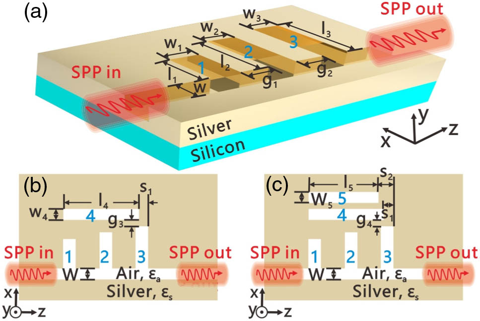
Figure 1.Schematic diagrams of the (a) THRC system, (b) FORC system, and (c) FIRC system.
When TM-polarized SPPs are injected from the left port of the THRC system, the propagating plasmonic waves confined to the metal-dielectric interface can directly couple into the three comb cavities [7]. As shown in Fig. 2(a), we can observe that two obvious transmission peaks, which are indicated by points B and D, exist in the transmission spectrum. It is noteworthy that dips are located on both sides of the peaks distinctly, which indicates the double PIT effects emerge in the transmission spectrum [7]. In order to get insight into the physical mechanism of the double PIT effects, the normalized magnetic field distributions of the transmission peaks and dips indicated by B, D and A, C, E are exhibited in Fig. 2. It can be found that it is the waveguide phase coupling between the cavities that gives rise to the peaks in the double PIT effects, while the reason for the appearance of the dips is related to the resonance of the cavities [6–9]. The theoretical results shown in Fig. 2(a) are calculated by using Eq. (B11) in Appendix B based on the CMT and TMM. It can be seen that the theoretical results basically agree with that simulated from the FDTD method. Notably, the suitable parameters (, , , , , and ) in Eq. (B11) are fitted by using the ANNs, and the detailed principle is presented in the next section. In addition, due to the extreme dispersion in the FR and PIT effect, the slow light, which is characterized by the group index , is shown in Fig. 2(b) [6–9]. Here, is the light velocity in vacuum, is the group delay, is the length between the source and monitor, and is the transmission phase shift [9]. It can be observed that two maximum group indices, 6.04 and 7.74, are achieved for the double PIT effects at the transparency peak wavelengths, 874 and 984 nm, respectively. Furthermore, we also calculate the dephasing times for the double PIT effects via , where is the reduced Planck’s constant and is the full width at half-maximum (FWHM) of the PIT effects [48,49]. For the THRC system, the dephasing times of the transmission peaks on the left (B) and that on the right () are estimated as 0.35 and 0.45 ps, respectively.

Figure 2.(a) Simulated transmission spectrum of the THRC system for Ag with loss (red solid line) and without loss (orange solid line), and theoretical transmission spectrum of the THRC system (blue dashed line); (b) group index and loss factor of the THRC system. The insets are simulated magnetic field distributions for the incident light at wavelengths of (A) 851 nm, (B) 893 nm, (C) 955 nm, (D) 1005 nm, and (E) 1048 nm.
The physical mechanism of the double PIT effects in the THRC system is relatively simple, which only takes the waveguide phase coupling into consideration. By contrast, we propose two relatively complex PWCCSs that include direct near-field coupling and indirect waveguide coupling simultaneously. In the FORC [Fig. 1(b)] and FIRC [Fig. 1(c)] systems, the rectangular cavities newly added in the structures are regarded as dark modes because they are excited by the comb cavities (bright mode) rather than the bus waveguide [47]. Here, the FDTD simulated transmission spectra (red solid line) and theoretical transmission spectra (blue circles) for the FORC and FIRC systems are depicted in Figs. 3(a) and 4(a), respectively. Compared with the FDTD-simulated results in Fig. 2(a), the optical characteristics around 1.18 μm in Figs. 3(a) and 4(a) become steep and asymmetric, indicating the appearance of the FRs [50]. Interestingly, the double PIT effects and the FRs simultaneously appear in the transmission spectrum, which is rarely mentioned in the related articles [6–9]. For the FRs in Figs. 3(a) and 4(a), the phase is dramatically changed [the transmittance varies sharply from the peak to dip with a small wavelength range of 12 nm (FORC) and 6 nm (FIRC)], which is suitable for the application of switches, sensors, slow light, and so on [51]. As shown in Figs. 3(b) and 4(b), the maximum group indices for the FORC and FIRC systems are 9.84 and 7.21, respectively. In addition, the dephasing times of the PIT peaks in the FORC and FIRC systems are similar to those in the THRC system because of the similar FWHM (–). Compared with the dephasing time of the single FR dip in the FORC system (0.42 ps), the double FR dips in the FIRC system have relatively larger values ( and ) due to the smaller FWHM. Obviously, the calculated dephasing times in this paper are larger than the general dephasing times of FR (on the order of 10 fs) [48,49].
Figure 3.(a) Simulated transmission spectrum of the FORC system for (red solid line) and 30 nm (orange solid line); theoretical transmission spectrum of the FORC system (blue circles); simulated transmission spectrum of the FORC system, which includes only cavities 1, 2, 4 (orange dashed line) and cavities 1, 2 (blue dashed line); (b) group index of the FORC system. The insets are calculated magnetic field distributions for the incident light at wavelengths of (A) 0.851 μm, (B) 0.893 μm, (C) 0.953 μm, (D) 1.01 μm, (E) 1.056 μm, (F) 1.168 μm, and (G) 1.18 μm.
Figure 4.(a) Simulated transmission spectrum of the FIRC system for (red solid line) and 60 nm (orange solid line); theoretical transmission spectrum of the FIRC system (blue dashed line); (b) group index of the FIRC system. The insets are calculated magnetic field distributions for the incident light at wavelengths of (A) 851 nm, (B) 893 nm, (C) 954 nm, (D) 1010 nm, (E) 1056 nm, (F) 1151 nm, (G) 1160 nm, (H) 1178 nm, and (I) 1189 nm.
In order to analyze the physical mechanism of the FR and PIT effects in the FORC system, the corresponding magnetic field distributions are shown in Fig. 3, where the plasmonic modes in the rectangular cavity are excited for the peak F and dip G collectively. In Fig. 3(a), the transmission spectra for the PWCCSs, which include only cavities 1, 2, 4 (orange dashed line) and cavities 1, 2 (blue dashed line), are identical. In addition, the FR becomes weak when coupling distance increases from 20 to 30 nm, while other peaks and dips are stable. We can infer that the destructive interference between the rectangular cavity 4 and comb cavity 3 gives rise to the transmission peak F because the near-field coupling among cavities 1, 2, and 4 is negligible. More importantly, the theoretical transmission spectrum calculated by using Eq. (B15) in Appendix B is quite approximate to the FDTD-simulated results. The fitted parameters in Eq. (B15) are , , , , , , , and (in THz for all parameters). For the FIRC system, the physical mechanism of the double FRs in Fig. 4(a) is similar to the single FR shown in Fig. 3(a), whereas the difference in the occurrences of the dips G and I is the resonance in cavities 5 and 4, respectively. From the magnetic field distributions F, G, H, and I shown in Fig. 4(a), it can be observed that it is the destructive interference between all the rectangular cavities in the FIRC system and the comb cavity 3 that forms the transmission peaks F and H, which is demonstrated by the fact that optical characteristics of the FRs become less steep when coupling distance is increased from 40 to 60 nm. Here, the theoretical results (blue dashed line) shown in Fig. 4(a) are calculated by using Eq. (B21) in Appendix B. In Eq. (B21), the fitted parameters predicted by ANNs are , , , , , , , , , and (in THz for all parameters). Here, since we do not take the higher order and lower order resonance modes in the cavities into consideration, the theoretically calculated results imperfectly match with the FDTD-simulated results.
3. SPECTRUM PREDICTION, INVERSE DESIGN, AND OPTIMIZATION FOR THE PWCCS
Mining the internal relationship between all structure parameters and electromagnetic response requires high computational cost to traverse all structure parameters (brute force) or to utilize the Monte Carlo (MC) method [20]. The efficiency of the device design and variability analysis will be improved if all simulation results are predictable based on a small sampling of simulation results. Machine-learning techniques, especially for ANNs, are data-driven methods that can predict the response for unknown data, for instance, based on classification, clustering, and regression [52]. More interestingly, it has been demonstrated that the trained ANNs can predict the same electromagnetic responses faster than conventional simulation methods [32,33]. Here, we use ANNs to predict the transmission spectrum for arbitrary structure parameters of PWCCSs. As shown in Fig. 5(a), the ANNs take the structure parameters (the dimension of the waveguide and cavities) as the input and predict the corresponding electromagnetic responses. For example, for the THRC system, the potential relationships between the structure parameters (the lengths, widths of the comb cavities 1, 2, 3, and the lengths of the gaps 1, 2 between the cavities) and the transmission spectrum are taken into consideration. Since the FORC and FIRC systems have more cavities than the THCR system, more structure parameters are input into the ANNs. The variation ranges of the structure parameters are fixed to be . Specifically, it means that the smallest length of the resonator 1 is 460 nm, and the largest one is 500 nm. In the FDTD simulations, the length of the resonator 1 is randomly generated from 460 to 500 nm with the precision of 1 nm. Repeated 2D FDTD simulations are employed to generate 20,000 different instances for eight parameters (, , , , , , , ) based on MC sampling [53]. It is noteworthy that the generation of the training and test instances, including structure parameters and the discrete data points in the simulated transmission spectrum, requires a significant amount of time. However, the prediction process for new instances is faster than conventional simulation methods because the weights and thresholds of ANNs are fixed once the training process is completed [32]. It takes us 30 h to generate 20,000 training instances with NVIDIA Tesla P100 GPU accelerators [54]. In order to guarantee the generalization of the training models, the ANNs are trained by using the 20,000 instances, while another 2000 instances are left as the test sets to validate the training effect. The model training of ANNs is done by optimizing the mean squared error based on the stochastic gradient descent (SGD) or adaptive moment estimation (Adam). Attempting to exhibit the performance of the trained ANNs, a simple indicator, score [55] is defined to measure the distance between the ANN-predicted results and the ground truth (FDTD simulations). In Eq. (1), relates to the total discrete data points in the FDTD-simulated transmission spectrum, and and are the discrete data points generated by utilizing the FDTD method and ANNs, respectively. The best and worst possible values of the score are 1.0 and arbitrary negative, respectively.
Figure 5.(a) Diagram of the ANNs applied in the spectrum prediction; (b) fitness for different generations in the spectrum prediction; (c) training losses for different iterations in the spectrum prediction; FDTD simulated transmission spectra and ANN-predicted transmission spectra for the (d) THRC, (e) FORC, and (f) FIRC systems; (g) fitness for different generations in the parameter fitting. The inset reveals the training losses for different iterations in the parameter fitting.
It should be noted that the network architecture and the selection of the hyperparameters determine the performance (prediction accuracy, convergence, and calculation time) of ANNs [42]. It is generally true that a high computation cost is taken to train the deep neural networks due to the existence of a huge number of weights between the neurons in different layers [52]. In order to ensure good accuracy and reduce training time, the GA is applied in optimizing the network architecture and selecting the hyperparameters (the algorithmic details of the GA are described in Appendix C). In the GA, the network architectures are fully connected, and four critical hyperparameters (number of layers, neurons per layer, the solvers for weights, and the activation functions for hidden layers) are regarded as the genetic genes. The score on the test sets is used as the fitness to evaluate each population’s accuracy. As shown in Fig. 5(b), the scores are increased evolutionally and level out at high levels, which indicates the optimizations for ANNs are efficient. After optimizing the network architectures based on the GA, the suitable hyperparameters for the THRC, FORC, and FIRC systems are [8-200-400-300-300-300-50-200-200, “relu,” “adam”], [12-400-200-300-400-100-200-200, “tanh,” “adam”], and [15-300-400-400-200-400-200, “relu,” “sgd”], respectively. Here, the input layers in the ANNs are the number of structure parameters, while the output layers match the discrete data points uniformly sampled from the transmission spectrum.
Due to the relatively simple network architecture, it takes a few minutes to train the ANNs by using the multilayer perception regressor (MLPRegressor) in the Scikit-learn library, which is a famous machine-learning toolbox for Python [55]. The other hyperparameters, such as L2 penalty, batch_size, max_iter, and tolerance, are set to , “auto,” 1000, and for all the PWCCSs. As shown in Figs. 5(b) and 5(c), for the THRC system, the score on the test sets is finally stabilized at 0.9862, and the training loss occasionally has sharp declines. This means that no matter the training sets or test sets, the predicted transmission spectra generated from the ANNs are very close to the simulation results calculated by the FDTD method. To illustrate the effectiveness of the spectrum prediction based on the ANNs, an arbitrary structure parameter is randomly selected from the test sets to make a comparative analysis between the ANNs’ predicted results and the FDTD simulation results. In Fig. 5(d), the red line relates to the FDTD-simulated transmission spectrum corresponding to the structure parameters (, , , , , , , and ), while the blue dots represent that predicted by the ANNs for the same structure parameters. It can be observed that the double PIT effects predicted by the ANNs match quite well with the FDTD-simulated transmission spectrum, even outside the training sets. Obviously, the trained ANNs not only fit the training data, but also learn some potential relationships between the structure parameters and the transmission spectrum for the THRC system. Similarly, the ANNs are also applied in spectrum prediction for the FORC and FIRC systems, and the comparison results are shown in Figs. 5(e) and 5(f), respectively. After many iterative rounds of model training, the scores on the test sets gradually rise to 0.9010 (FORC) and 0.9538 (FIRC), which indicates that the ANNs can effectively predict the transmission spectra for the relatively complex PWCCSs. In Figs. 5(e) and 5(f), the ANN-predicted transmission spectra and the FDTD-simulated transmission spectra are broadly similar, though the similarity for the steep optical characteristics (such as the FR) is imperfect. The reason for this imperfection is attributed to the insufficiency of the training data and the relatively simple network architectures. Actually, we can improve the precision of spectrum prediction by adding training data or designing complex network architecture. However, it is at the cost of training time and power, and the overfitting problem is difficult to avoid [56,57].
In addition, when the physical phenomena in the PWCCSs are theoretically analyzed, there are many theoretical parameters needing to be addressed by using the data-fitting method. It is more beneficial to automatically determine the theoretical parameters for a specific electromagnetic response because the data fitting is an empirical and tedious process. We use ANNs to search the suitable parameters for the theoretical models in Appendix B, and it consists of the following steps: (i) 20,000 training instances, which include the theoretical parameters and 200 discrete data points in the theoretically calculated transmission spectrum are generated by utilizing the MC method. It only takes a few seconds to generate the training sets because the computing process for theoretical models is not complex. (ii) In order to optimize the network architectures of the ANNs, we also use the GA to select the suitable hyperparameters. In Fig. 5(g), it can be observed that the evolutionary scores are maintained at a higher level from the first generation because the theoretical models behind the physical phenomenon really exist. (iii) We select three excellent ANNs whose scores on the test sets are greater than 99.60% to predict the fitting parameters for the FDTD-simulated transmission spectra, and the inset in Fig. 5(g) reveals the variation tendency of the loss in the model training. In Figs. 2(a), 3(a), and 4(a), the similarity between the theoretically calculated transmission spectra and the FDTD transmission spectra demonstrates the ANNs can predict the fitting parameters for the theoretical models.
For the PWCCSs shown in Fig. 1, the inverse design based on ANNs is also analyzed here. For this purpose, we should design an arbitrary transmission spectrum within reasonable limits, and the ANNs could predict the structure parameters that would most closely produce the artificial transmission spectrum. Compared with the “forward” ANNs, which have applications in the spectrum prediction (from structure parameters to transmission spectrum), an “inverse” network architecture that reproduces the structure parameters from the transmission spectrum is specially constructed. As shown in Fig. 6(a), the inputs and outputs of the inverse network architecture are the discrete points uniformly sampled from the transmission spectrum and the structure parameters of the PWCCSs, respectively. Similarly, the inverse ANNs are trained by using the 20,000 training instances, and the network architectures are optimized by utilizing the GA. After a few iterative evolution steps, the suitable network architectures and hyperparameters of the inverse ANNs for the THRC, FORC, and FIRC systems are [200-200-400-400-8, “relu,” “sgd”], [200-200-400-300-100-12, “relu,” “adam”], and [200-300-300-300-200-15, “relu,” “adam”], respectively. Compared with the THRC system, the inverse design for the FORC and FIRC systems requires more sophisticated network architecture because more structure parameters must be predicted. The effectiveness of the inverse design for the THRC, FORC, and FIRC systems is quantitatively validated by calculating the score on the test sets. After a few iterative training steps, the score reaches 0.912, 0.943, and 0.896 for the THRC, FORC, and FIRC systems, respectively. In order to provide a vivid visualization of the inverse design effect for the PWCCSs, the FDTD-simulated transmission spectra randomly selected from the test sets are input into the ANNs. The red circles in Figs. 6(b)–6(d) show the real structure parameters, while the blue circles relate to the inverse ANN-predicted structure parameters. For the sake of convenience, the structure parameters are normalized to a range from 0 to 1. Interestingly, it can be observed that most of the predicted structure parameters agree with the real structure parameters accurately. To consider the influence of prediction error, the insets in Figs. 6(b)–6(d) depict the FDTD-simulated transmission spectra corresponding to the real structure parameters (red lines) and predicted structure parameters (blue dots) for the THRC, FORC, and FIRC systems, respectively. Compared with the FDTD results, it can be found that the structure parameters predicted by the ANNs can reproduce transmission spectra with a high similarity. Obviously, it no doubt provides a new way to train ANNs for the inverse design of PWCCSs.
Figure 6.(a) Diagram of the ANNs applied in the inverse design and performance optimization problems; comparison results between the real structure parameters and ANN-predicted structure parameters for the (b) THRC, (c) FORC, and (d) FIRC systems. The insets in (b)–(d) are the FDTD-simulated transmission spectra corresponding to the real structures (red solid line) and ANN-predicted structure parameters (blue dashed line); (e) transmittance optimization for the THRC system; (f) bandwidth optimization for the FORC system; (g) transmittance optimization for the FIRC system.
Similar to the inverse design, the ANNs can be applied in optimizing for a specific property of PWCCSs, such as transmittance, bandwidth, and FWHM. In order to validate the performance optimization of the transmittance for an arbitrary wavelength and avoid generating unreasonable results, the transmission spectrum randomly selected from the test sets is shifted manually for the THRC system. The blue solid line and red solid line in Fig. 6(e) are the FDTD-simulated transmission spectrum and the redshifted transmission spectrum, respectively. It can be observed that the transmittance at 900 nm increases from 0.05 to 0.68 by shifting the transmission spectrum. The redshifted transmission spectrum is input into the inverse ANNs, and the most probable structure parameters are predicted by the ANNs. The black dashed line in Fig. 6(e) represents the FDTD-simulated result corresponding to the structure parameters predicted by the inverse ANN (, , , , , , , and , all in nm). Obviously, the transmittance optimization for a given wavelength can be achieved by using ANNs due to the similarity between the ANN-predicted transmission spectrum and the redshifted transmission spectrum. For the redshifted transmission spectrum, we have compared the algorithmic performance between the ANNs and two representative evolutionary algorithms [GA and particle swarm optimization (PSO)]. Please see the comparative analysis in Appendix D. Moreover, we try to optimize the bandwidth of the optical channel in the double PIT effects or FR based on the ANNs. For the FORC system, we expect to further reduce the bandwidth of the FR to achieve much steeper optical characteristics. For this purpose, the transmission spectrum is designed optimally [blue line in Fig. 6(f)], especially for the bandwidth of the FR (the bandwidth between the peak and dip of the FR is reduced from 12 to 8 nm). Then, the optimized transmission spectrum is input into the ANNs, and the predicted structure parameters are , , , , , , , , , , , and (in nm for all parameters). Here, the black dots in Fig. 6(f) represent the FDTD simulation results calculated for the predicted structure parameters. As shown in Fig. 6(f), the FDTD-simulated results are close to the optimized transmission spectrum, which indicates the feasibility for bandwidth optimization by using the ANNs. Besides, the transmittance of the transmission spectrum for the FIRC system is also optimized. The red line in Fig. 6(g) is the original transmission spectrum randomly selected from the test sets for the FIRC system, and the blue line is the manually blueshifted transmission spectrum. Here, the transmission spectrum in a given wavelength range (700–1300 nm) can be shifted to achieve steeper optical characteristics or higher transmittance. When the blueshifted transmission spectrum is input into the inverse ANNs, the structure parameters (, , , , , , , , , , , , , , , and , all in nm) are predicted quickly. Apparently, the blueshifted transmission spectrum agrees well with the FDTD-simulated transmission spectrum (black dotted line) calculated for the predicted structure parameters, which realizes the transmittance optimization for a specific wavelength in the FIRC system.
Finally, we should consider the influence of the training set size on the performance of the ANNs because generating the training instances takes significant effort, especially for the method based on 3D FDTD simulation. Here, we calculate the prediction accuracies for different numbers of training instances in the spectrum prediction and inverse design; the calculated results are shown in Fig. 7. It should be noted that we select the previously optimized ANNs whose prediction accuracies (scores) exceed 90% when the training set size is 20,000 to illustrate the influence of different training set sizes. As shown in Fig. 7, all the prediction accuracies are improved when the number of training instances increases from 5000 to 12,000, which indicates that the extension of training sets is beneficial to the accuracy. More importantly, the scores for the THRC system (eight structure parameters) are larger than those of the FORC system (12 structure parameters) and FIRC system (15 structure parameters) with the same training set size. This means that the more targeted the structure parameters are, the larger the training set size needed. Thus, if a large number of structural parameters need to be predicted, we should appropriately increase the number of training instances or design a more complex network architecture of ANNs to ensure accuracy. To be sure, generating the training instances is an ineluctable problem for all supervised machine learning, including the ANN-based method. In Ref. [32], Peurifoy et al. pointed out two reasons why this method is still very useful, even though a certain amount of training instances are necessary. We would add two further reasons why we believe the method is valuable. First, once the ANN-based model is constructed, we can obtain the predicted results orders of magnitude faster than conventional simulations. For example, for the same inverse design problem, the required time of the ANNs is longer than that of the GA and PSO (12 h) because it takes 30 h to generate the training instances and to train the model. However, if we have three different transmission spectra that need to be inversely designed, it spends 36 h on iterative optimization based on GA or PSO. Then, the advantage in time of GA and PSO is not obvious because the ANNs-based model is reusable once the model is constructed. Second, many photonic devices, especially for plasmonic devices (plasmonic waveguide systems, gratings, and so on) and photonic crystals, are usually calculated numerically based on 2D FDTD simulation. The ANN-based method is very suitable for applications in these photonic devices, which can be simulated by 2D FDTD simulation due to the short time in generating training instances.
Figure 7.Prediction accuracies for different numbers of training instances in the (a) spectrum prediction and (b) inverse design.
4. CONCLUSION
In this paper, we proposed a novel method using ANNs to achieve spectrum prediction, inverse design, and performance optimization for PWCCSs. The FR and PIT effects originating from mode coupling in PWCCSs were explained theoretically and taken as the example to verify the effectiveness of ANNs. The uncertain parameters in the theoretical models were fitted by using the ANNs effectively. In order to ensure good accuracy and reduce training time, we used the GA to design the network architectures and select the suitable hyperparameters for ANNs. It is important to note that the transmission spectrum predicted by ANNs is approximate to the FDTD-simulated results with high precision. More importantly, the ANNs have been successfully employed in solving the inverse design and performance optimization problems for PWCCSs. Obviously, we constructed a novel model-driven analysis method for PWCCSs, which are expected to have significant applications in the design, analysis, and optimization of optical devices.
References
[1] D. K. Gramotnev, S. I. Bozhevolnyi. Plasmonics beyond the diffraction limit. Nat. Photonics, 4, 83-91(2010).
[2] S. Zhang, D. A. Genov, Y. Wang, M. Liu, X. Zhang. Plasmon-induced transparency in metamaterials. Phys. Rev. Lett., 101, 047401(2008).
[3] A. B. Khanikaev, C. Wu, G. Shvets. Fano-resonant metamaterials and their applications. Nanophotonics, 2, 247-264(2013).
[4] T. Zhang, J. Dai, Y. Dai, Y. Fan, X. Han, J. Li, F. Yin, Y. Zhou, K. Xu. Dynamically tunable plasmon induced absorption in graphene-assisted metallodielectric grating. Opt. Express, 25, 26221-26233(2017).
[5] T. Zhang, J. Dai, Y. Dai, Y. Fan, X. Han, J. Li, F. Yin, Y. Zhou, K. Xu. Tunable plasmon induced transparency in a metallodielectric grating coupled with graphene metamaterials. J. Lightwave Technol., 35, 5142-5149(2017).
[6] R. D. Kekatpure, E. S. Barnard, W. Cai, M. L. Brongersma. Phase-coupled plasmon-induced transparency. Phys. Rev. Lett., 104, 243902(2010).
[7] H. Lu, X. Liu, D. Mao. Plasmonic analog of electromagnetically induced transparency in multi-nanoresonator-coupled waveguide systems. Phys. Rev. A, 85, 053803(2012).
[8] Z. He, H. Li, S. Zhan, G. Cao, B. Li. Combined theoretical analysis for plasmon-induced transparency in waveguide systems. Opt. Lett., 39, 5543-5546(2014).
[9] X. Han, T. Wang, X. Li, B. Liu, Y. He, J. Tang. Ultrafast and low-power dynamically tunable plasmon-induced transparencies in compact aperture-coupled rectangular resonators. J. Lightwave Technol., 33, 5133-5139(2015).
[10] H. Li, L. Wang, J. Liu, Z. Huang, B. Sun, X. Zhai. Investigation of the graphene based planar plasmonic filters. Appl. Phys. Lett., 103, 211104(2013).
[11] X. Han, T. Wang, X. Li, S. Xiao, Y. Zhu. Dynamically tunable plasmon induced transparency in a graphene-based nanoribbon waveguide coupled with graphene rectangular resonators structure on sapphire substrate. Opt. Express, 23, 31945-31955(2015).
[12] H. Lu, X. Gan, D. Mao, J. Zhao. Graphene-supported manipulation of surface plasmon polaritons in metallic nanowaveguides. Photon. Res., 5, 162-167(2017).
[13] L. Chen, T. Zhang, X. Li, W. P. Huang. Novel hybrid plasmonic waveguide consisting of two identical dielectric nanowires symmetrically placed on each side of a thin metal film. Opt. Express, 20, 20535-20544(2012).
[14] Y. Zhu, X. Hu, H. Yang, Q. Gong. On-chip plasmon-induced transparency based on plasmonic coupled nanocavities. Sci. Rep., 4, 3752(2014).
[15] Z. Chai, X. Hu, Y. Zhu, S. Sun, H. Yang, Q. Gong. Ultracompact chip-integrated electromagnetically induced transparency in a single plasmonic composite nanocavity. Adv. Opt. Mater., 2, 320-325(2014).
[16] Z. Chai, X. Hu, H. Yang, Q. Gong. All-optical tunable on-chip plasmon-induced transparency based on two surface-plasmon-polaritons absorption. Appl. Phys. Lett., 108, 151104(2016).
[17] H. A. Haus. Waves and Fields in Optoelectronics(1984).
[18] X. Han, T. Wang, B. Liu, Y. He, Y. Zhu. Tunable triple plasmon-induced transparencies in dual T-shaped cavities side-coupled waveguide. IEEE Photon. Technol. Lett., 28, 347-350(2016).
[19] Z. Chen, L. Yu. Multiple Fano resonances based on different waveguide modes in a symmetry breaking plasmonic system. IEEE Photon. J., 6, 4802208(2014).
[20] S. Inampudi, H. Mosallaei. Neural network based design of metagratings. Appl. Phys. Lett., 112, 241102(2018).
[21] L. F. Frellsen, Y. Ding, O. Sigmund, L. H. Frandsen. Topology optimized mode multiplexing in silicon-on-insulator photonic wire waveguides. Opt. Express, 24, 16866-16873(2016).
[22] A. Y. Piggott, J. Lu, K. G. Lagoudakis, J. Petykiewicz, T. M. Babinec, J. Vučković. Inverse design and demonstration of a compact and broadband on-chip wavelength demultiplexer. Nat. Photonics, 9, 374-377(2015).
[23] B. Shen, P. Wang, R. Polson, R. Menon. An integrated-nanophotonics polarization beamsplitter with 2.4 × 2.4 μm2 footprint. Nat. Photonics, 9, 378-382(2015).
[24] H. Cui, X. Sun, Z. Yu. Genetic-algorithm-optimized wideband on-chip polarization rotator with an ultrasmall footprint. Opt. Lett., 42, 3093-3096(2017).
[25] J. C. Mak, C. Sideris, J. Jeong, A. Hajimiri, J. K. Poon. Binary particle swarm optimized 2 × 2 power splitters in a standard foundry silicon photonic platform. Opt. Lett., 41, 3868-3871(2016).
[26] Z. Lin, X. Liang, M. Lončar, S. G. Johnson, A. W. Rodriguez. Cavity-enhanced second-harmonic generation via nonlinear-overlap optimization. Optica, 3, 233-238(2016).
[27] T. W. Hughes, M. Minkov, I. A. Williamson, S. Fan. Adjoint method and inverse design for nonlinear nanophotonic devices. ACS Photon., 5, 4781-4787(2018).
[28] Z. Yu, H. Cui, X. Sun. Genetically optimized on-chip wideband ultracompact reflectors and Fabry-Perot cavities. Photon. Res., 5, B15-B19(2017).
[29] E. Bor, C. Babayigit, H. Kurt, K. Staliunas, M. Turduev. Directional invisibility by genetic optimization. Opt. Lett., 43, 5781-5784(2018).
[30] P.-H. Fu, S.-C. Lo, P.-C. Tsai, K.-L. Lee, P.-K. Wei. Optimization for gold nanostructure-based surface plasmon biosensors using a microgenetic algorithm. ACS Photon., 5, 2320-2327(2018).
[31] G. Carleo, M. Troyer. Solving the quantum many-body problem with artificial neural networks. Science, 355, 602-606(2017).
[32] J. Peurifoy, Y. Shen, L. Jing, Y. Yang, F. Canorenteria, B. Delacy, M. Tegmark, J. D. Joannopoulos, M. Soljacic. Nanophotonic particle simulation and inverse design using artificial neural networks. Sci. Adv., 4, eaar4206(2018).
[33] K. Kojima, B. Wang, U. Kamilov, T. Koike-Akino, K. Parsons. Acceleration of FDTD-based inverse design using a neural network approach. Integrated Photonics Research, Silicon and Nanophotonics, ITu1A.4(2017).
[34] D. Liu, Y. Tan, E. Khoram, Z. Yu. Training deep neural networks for the inverse design of nanophotonic structures. ACS Photon., 5, 1365-1369(2018).
[35] M. H. Tahersima, K. Kojima, T. Koike-Akino, D. Jha, B. Wang, C. Lin, K. Parsons. Deep neural network inverse design of integrated nanophotonic devices(2018).
[36] W. Ma, F. Cheng, Y. Liu. Deep-learning enabled on-demand design of chiral metamaterials. ACS Nano, 12, 6326-6334(2018).
[37] I. Malkiel, A. Nagler, M. Mrejen, U. Arieli, L. Wolf, H. Suchowski. Deep learning for design and retrieval of nano-photonic structures(2017).
[38] R. R. Andrawis, M. A. Swillam, M. A. El-Gamal, E. A. Soliman. Artificial neural network modeling of plasmonic transmission lines. Appl. Opt., 55, 2780-2790(2016).
[39] M. Turduev, E. Bor, C. Latifoglu, I. H. Giden, Y. S. Hanay, H. Kurt. Ultra-compact photonic structure design for strong light confinement and coupling into nano-waveguide. J. Lightwave Technol., 36, 2812-2819(2018).
[40] E. Bor, O. Alparslan, M. Turduev, Y. S. Hanay, H. Kurt, S. I. Arakawa, M. Murata. Integrated silicon photonic device design by attractor selection mechanism based on artificial neural networks: optical coupler and asymmetric light transmitter. Opt. Express, 26, 29032-29044(2018).
[41] Z. Liu, D. Zhu, S. P. Rodrigues, K.-T. Lee, W. Cai. A generative model for inverse design of metamaterials(2018).
[42] B. Baker, O. Gupta, N. Naik, R. Raskar. Designing neural network architectures using reinforcement learning(2016).
[43] K. O. Stanley, R. Miikkulainen. Evolving neural networks through augmenting topologies. Evol. Comput., 10, 99-127(2002).
[44] B. Shahriari, K. Swersky, Z. Wang, R. P. Adams, N. De Freitas. Taking the human out of the loop: a review of Bayesian optimization. Proc. IEEE, 104, 148-175(2016).
[45] B. Zoph, Q. V. Le. Neural architecture search with reinforcement learning(2016).
[46] T. Wang, Y. Zhang, Z. Hong, Z. Han. Analogue of electromagnetically induced transparency in integrated plasmonics with radiative and subradiant resonators. Opt. Express, 22, 21529-21534(2014).
[47] Z. Zhang, L. Zhang, H. Li, H. Chen. Plasmon induced transparency in a surface plasmon polariton waveguide with a comb line slot and rectangle cavity. Appl. Phys. Lett., 104, 231114(2014).
[48] A. Ahmadivand, R. Sinha, B. Gerislioglu, M. Karabiyik, N. Pala, M. Shur. Transition from capacitive coupling to direct charge transfer in asymmetric terahertz plasmonic assemblies. Opt. Lett., 41, 5333-5336(2016).
[49] M. Qin, L. Wang, X. Zhai, D. Chen, S. Xia. Generating and manipulating high quality factors of Fano resonance in nanoring resonator by stacking a half nanoring. Nano. Res. Lett., 12, 578(2017).
[50] H. Lu, X. Liu, D. Mao, G. Wang. Plasmonic nanosensor based on Fano resonance in waveguide-coupled resonators. Opt. Lett., 37, 3780-3782(2012).
[51] C. Wu, A. B. Khanikaev, G. Shvets. Broadband slow light metamaterial based on a double-continuum Fano resonance. Phys. Rev. Lett., 106, 107403(2011).
[52] Y. LeCun, Y. Bengio, G. Hinton. Deep learning. Nature, 521, 436-444(2015).
[53] G. Fishman. Monte Carlo: Concepts, Algorithms, and Applications(2013).
[54] A. Devarakonda, M. Naumov, M. Garland. AdaBatch: adaptive batch sizes for training deep neural networks(2017).
[55] .
[56] Y. Shen, N. C. Harris, S. Skirlo, M. Prabhu, T. Baehr-Jones, M. Hochberg, X. Sun, S. Zhao, H. Larochelle, D. Englund, M. Soljačić. Deep learning with coherent nanophotonic circuits. Nat. Photonics, 11, 441-446(2017).
[57] G. C. Cawley, N. L. Talbot. On over-fitting in model selection and subsequent selection bias in performance evaluation. J. Mach. Learn. Res., 11, 2079-2107(2010).
[58] P. B. Johnson, R. Christy. Optical constants of the noble metals. Phys. Rev. B, 6, 4370-4379(1972).
[59] A. Chipperfield, P. Fleming. The MATLAB genetic algorithm toolbox. IEEE Colloquium on Applied Control Techniques Using MATLAB(1995).
[60] P. Ghamisi, J. A. Benediktsson. Feature selection based on hybridization of genetic algorithm and particle swarm optimization. IEEE Geosci. Remote Sens. Lett., 12, 309-313(2015).
[61] A. da Silva Ferreira, C. H. da Silva Santos, M. S. Gonçalves, H. E. H. Figueroa. Towards an integrated evolutionary strategy and artificial neural network computational tool for designing photonic coupler devices. Appl. Soft Comput., 65, 1-11(2018).


