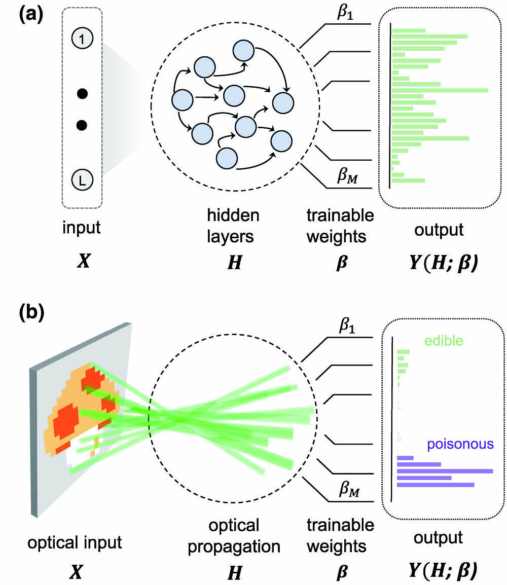
Fig. 1. Schematic architecture of the photonic extreme learning machine (PELM). (a) General ELM scheme with the input data set X, which is fed into a reservoir and gives out the hidden-layer output matrix H. The trainable readout weights βi determine the network output Y=Y(H;β). (b) In the optical case, the input (a mushroom in the example) is encoded on the optical field, and hidden neurons have been replaced by modes that interact during propagation. Training of the photonic classifier is enabled by M detection channels.

Fig. 2. Learning ability of the PELM architecture. The optical computing scheme is evaluated on the MNIST data set by varying the encoding properties and feature space. (a) Input digit and 2D phase mask showing its encoding by noise embedding: the input signal overlaps with a disordered matrix. PELM training and testing error for noise embedding when varying the (b) noise amplitude and (c) its correlation length, for M=1600. (d) Input vector encoded over a carrier signal (Fourier embedding). (e) Classification error versus the number of frequencies of the embedding signal. (f) Minimum testing error with the increasing number of features M. The indicated accuracies are the best ones reported with random ELM (rELM) [47], random projections (RP) [41], and kernel ELM (kELM) [47] on the same task.

Fig. 3. Experimental implementation. (a) Sketch of the optical setup. A phase-only spatial light modulator (SLM) encodes data on the wavefront of a 532 nm continuous-wave laser. The far field in the lens focal plane is imaged on a camera. Insets show a false-color embedding matrix and training data encoded as phase blocks, respectively. (b) Detected spatial intensity distribution for a given input sample. White-colored areas reveal camera saturation in high-intensity regions, which provides the network nonlinear function. Pink boxes show some of the M spatial modes (blocks of pixels) that are used as readout channels. (c) Example of an input data in a feature space of dimension M=256, as projected by the optical device. Each bar represents an output channel, and training consists in finding the vector that properly tunes all the bar heights.

Fig. 4. Experimental performance of the PELM on classification and regression tasks. Confusion matrices on the MNIST data set for a free-space PELM, which makes use of (a) Fourier and (b) random embedding (92.18% and 92.06% accuracy, M=4096). (c) Performance on the mushroom binary classification problem (95.4%). (d) Optical predictions and true values for the abalone data set. (e) Classification and (f) regression error as a function of the number of features. Rapid convergence to optimal performance is found. Experimental results are compared with numerical simulations and training errors.